Download
1 / 26
420 likes | 882 Views
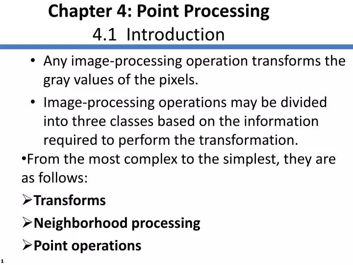
Chapter 4: Point Processing 4.1 Introduction. From the most complex to the simplest, they are as follows: Transforms Neighborhood processing Point operations. Any image-processing operation transforms the gray values of the pixels.

E N D
Chapter 4: Point Processing4.1 Introduction • From the most complex to the simplest, they are as follows: • Transforms • Neighborhood processing • Point operations Any image-processing operation transforms the gray values of the pixels. Image-processing operations may be divided into three classes based on the information required to perform the transformation.
FIGURE 4.1 (Point operations)
4.2 Arithmetic Operations These operations act by applying a simple function ex: y=x±C, y=Cx In each case we may have to adjust the output slightly in order to ensure that the results are integers in the 0 . . . 255 range (type uint8)
4.2 Arithmetic Operations • COMPLEMENTS • The complement of a grayscale imageis its photographic negative • type double (0.0~1.0):1-m • type uint8 • (0~255): 255-m
4.3 Histograms • A graph indicating the number of times each gray level occurs in the image • >>imhistfunction • a = [10 10 10 10 10; • 20 20 20 20 10; • 50 50 50 50 50; • 90 90 90 50 50]
4.3.1 Histogram Stretching • A table of the numbers ni of gray values • (with n = 360, as before) • We can stretch out the gray levels in the center of the range • by applying • the piecewise • linear function
4.3.1 Histogram Stretching • where i is the original gray level and j is its result after the transformation • This function has the effect of stretching the gray levels 5–9 to gray levels 2–14 • The corresponding histogram
FIGURE 4.10 • Use of imadjust • imadjustis designed to work equally well on images of type double, uint8, or uint16 • the values of a, b, c, and d must be between 0 and 1 • the function automatically converts the image im (if needed) to be of type double
4.3.1 Histogram Stretching • Note that imadjust does not work quite in the same way as shown in Figure 4.9 • The imadjust function has one other optional parameter: the gamma value
4.3.1 Histogram Stretching • A PIECE WISE LINEAR-STRETCHING FUNCTION • The heart of this function will be the lines whereim is the input image and out is the output image
FIGURE 4.16 Refer to figure 4.15 The tire image after piecewise linear-stretching and piecewise linear-stretching function.
Function histpwl N=length(a); out=zeros(size(im)); for i=1:N-1 pix=find(im>=a(i) & im<a(i+1)); out(pix)=(im(pix)-a(i))*(b(i+1)-b(i))/(a(i+1)-a(i))+b(i); end pix=find(im==a(N)); out(pix)=b(N); if classChanged==1 out = uint8(255*out); end function out = histpwl(im,a,b) % % HISTPWL(IM,A,B) applies a piecewise linear transformation to the pixel values % of image IM, where A and B are vectors containing the x and y coordinates % of the ends of the line segments. IM can be of type UINT8 or DOUBLE, % and the values in A and B must be between 0 and 1. % % For example: % % histpwl(x,[0,1],[1,0]) % % simply inverts the pixel values. % classChanged = 0; if ~isa(im, 'double'), classChanged = 1; im = im2double(im); end if length(a) ~= length (b) error('Vectors A and B must be of equal size'); end
4.3.2 Histogram Equalization • An entirely automatic procedure • Suppose our image has L different gray levels, 0, 1, 2, . . . , L − 1, and gray level i occurs nitimes in the image • Where n=n0 +n1 +n2 +· · ·+nL−1 • EXAMPLE Suppose a 4-bit grayscale image has the histogram shown in Figure 4.17, associated with a table of the numbers ni of gray values
4.3.2 Histogram Equalization (L-1)/n
FIGURE 4.19 • histeq
4.3.2 Histogram Equalization • WHY IT WORKS If we were to treat the image as a continuous function f (x, y)and the histogram as the area between different contours, then we can treat the histogram • as a probability density • function.
4.4 Lookup Tables • Point operations can be performed very effectively by using a lookup table, known more simply as an LUT • e.g., the LUTcorresponding to division by 2 looks like • If T is a lookup table in MATLAB and im is our image, the lookup table can be applied by the simple command
4.4 Lookup Tables • e.g., >> b = b+1; • As another example, suppose we wish to apply an LUT to implement the contrast-stretching function >> b2 = T(b+1);