Laplace Transforms

1. Chapter 3 Laplace Transforms 1.Standard notation in dynamics and control (shorthand notation) 2. Converts mathematics to algebraic operations 3. Advantageous for block diagram analysis

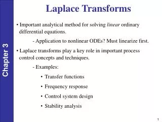
2. Laplace Transforms • Important analytical method for solving linear ordinary differential equations. • - Application to nonlinear ODEs? Must linearize first. • Laplace transforms play a key role in important process control concepts and techniques. • - Examples: • Transfer functions • Frequency response • Control system design • Stability analysis

3. Definition The Laplace transform of a function, f(t), is defined as where F(s) is the symbol for the Laplace transform, L is the Laplace transform operator, and f(t) is some function of time, t. Note: The L operator transforms a time domain function f(t) into an s domain function, F(s). s is a complex variable: s = a + bj,

4. Inverse Laplace Transform, L-1: By definition, the inverse Laplace transform operator, L-1, converts an s-domain function back to the corresponding time domain function: Important Properties: Both L and L-1 are linear operators. Thus,

5. where: - x(t) and y(t) are arbitrary functions - a and b are constants - Similarly,

6. Laplace Transforms of Common Functions • Constant Function • Let f(t) = a (a constant). Then from the definition of the Laplace transform in (3-1),

7. Step Function • The unit step function is widely used in the analysis of process control problems. It is defined as: Because the step function is a special case of a “constant”, it follows from (3-4) that

8. Derivatives • This is a very important transform because derivatives appear in the ODEs we wish to solve. In the text (p.53), it is shown that initial condition at t = 0 Similarly, for higher order derivatives:

9. where: - n is an arbitrary positive integer - Special Case: All Initial Conditions are Zero Suppose Then In process control problems, we usually assume zero initial conditions. Reason: This corresponds to the nominal steady state when “deviation variables” are used, as shown in Ch. 4.

10. Exponential Functions • Consider where b > 0. Then, • Rectangular Pulse Function • It is defined by:

11. Impulse Function (or Dirac Delta Function) • The impulse function is obtained by taking the limit of the • rectangular pulse as its width, tw, goes to zero but holding • the area under the pulse constant at one. (i.e., let ) • Let, • Then,

12. Time, t The Laplace transform of the rectangular pulse is given by

13. Other Transforms Note: Chapter 3

14. Difference of two step inputs S(t) – S(t-1) (S(t-1) is step starting at t = h = 1) By Laplace transform Chapter 3 Can be generalized to steps of different magnitudes (a1, a2).

15. Table 3.1. Laplace Transforms • See page 54 of the text.