Download
1 / 26
260 likes | 394 Views
A Numerical Model to Investigate Urban Pollution. S. D. Wright, L. Elliott and D.B. Ingham The School of the Environment University of Leeds, England. To develop a numerical model to calculate the ABL within the urban environment To use real orography and land-use data-sets

E N D
A Numerical Model to Investigate Urban Pollution S. D. Wright, L. Elliott and D.B. Ingham The School of the Environment University of Leeds, England
To develop a numerical model to calculate the ABL within the urban environment To use real orography and land-use data-sets To develop a model applicable to any area of the United Kingdom For the model to be easy to use To use the model to investigate urban pollution From the National Environmental Research Council (NERC) thematic programme: “Urban regeneration and the environment” Urgent An extension of research funded by the British Textile Technology Group (BTTG) responsible for monitoring industrial emissions in the north of England Aims of the Research Aims Motivation
Physics Included in the Model • Governing equations: • Reynolds averaged Navier-stokes equations • Potential temperature (stratified flow) • Turbulent properties • Equations for TKE and rate of dissipation of TKE (k & ) • Used to form a non-isotropic algebraic stress model • Radiation model • Annual and diurnal radiation model • Force-restore method at the surface • Urban effects • Urban drag parameterisation using real topography and land-use data • Thermal effects included within the radiation model
Numerical Techniques • Solution domain • Fully 3D and time dependent • Resolution from all of the UK 20x20km • Use an embedded mesh technique to resolve a specific urban conurbation • Solution technique • A finite volume discretisation of the governing equations including a QUICK advection scheme • A Poisson equation for pressure based on the SIMPLEC algorithm • Uses a Tri-Diagonal Matrix Algorithm (TDMA) • Turbulent stresses are explicitly included within the model (allows many different turbulence schemes to be implemented)
Formulation of the Lower Boundary Topography • A data set provides heights above sea level at 500 metre resolution • These heights are interpolated onto a stretched mesh refined around the conurbation of interest • Several embedded meshes are included to gain the required resolution of the urban conurbation
Formulation of the Lower Boundary Categorisations Land use • A data set is used to categorise the land use at each point in the mesh • For each of the 26 categories, the percentage of cover per 1km square is calculated • This is used to formulate boundary conditions for the model and to identify areas of urbanisation
The Numerical Model • The model is fully interactive with no specialised knowledge needed. • All aspects of the model can be manipulated from the graphical user interface • The G.U.I. is used to manipulate the two data sets and the numerical model
Modelling the turbulence within the Atmospheric Boundary-layer is the most difficult aspect facing the numerical modeller • In the numerical model this has been achieved by implementing two well known sophisticated turbulence models: • The k- model • The algebraic stress model • The model can be chosen from a pull-down menu
Depending on the facilities available the resolution of the simulation can be altered by increasing or decreasing the horizontal and vertical mesh sizes • In general, the greater the mesh size the better the resolution, but the slower the calculation will be • The refinement point, i.e. the area of interest can be altered by the mouse sensitive screen • The refinement point in the figure opposite can be seen to be in the centre of the display
Through pull down menus the model can be tailored to model the air flow in any region of the United Kingdom. • Here, the properties of the 3D calculation are being altered. Relaxation parameters adjust the efficiency of the calculation with correct choices leading to drastic improvements in the solution time
The number of embedded meshes can also be adjusted • The more embedded meshed then the better the resolution of the solution but the slower the simulation • The number of embedded meshes can be adjusted using the slider control on the main interface
Once the number of embedded meshes has been chosen then each embedded mesh needs to be defined • Each mesh can be defined individually by using the mouse sensitive screen • Alternatively on Auto-mesh function exists that defines the meshes given the final refinement point
Once the solution domain has been defined the land-use properties in the region of interest can be examined • Each of the 26 land-use categories can be individually examined to make sure the solution domain represents the area of interest
The percentage per unit area of and chosen land-use can be examined • For example in the figure opposite all urban conurbations at a resolution of more than 50% per unit area will be displayed • The embedded meshes can be refined, if necessary, at any time
It is possible to display the data (land-use and relief height) in a variety of different formats • 2D and 3D plotting functions are available that show just the relief height or superimpose the land-use onto the relief height maps
Here the urban land-use at 50% resolution is shown for the seventh embedded mesh of the solution domain • This figure shows the resolution that is possible by using the two data-sets • In this figure, the conurbations of Leeds Manchester, Liverpool and Birmingham, as well as others, are visible
It is possible to save and restore simulations at any point • It is also possible to print any or all of the displays with the G.U.I. at any time
Here a simulation has been restored with 4 embedded meshes, with 240 time-steps of 5 minutes • It is possible to move forwards and backwards through the simulation, viewing any results already obtained
Menus are available to adjust the format of the results to be examined • 3D plots are used to view the simulations, similar to the one shown earlier, with flow vectors and surface contouring implemented • The vectors and surface contours can be shaded according to one of many flow properties (shown in the figure)
Vectors can be restricted to a 2D slice through the simulation domain, for clarity • Full 3D vector plots are also available with the number of vectors in the horizontal and vertical directions adjustable
The figure opposite shows a typical flow plot • The surface shading, showing contours of surface pressure, indicates that there is high surface pressure in the region of the Pennines and North Wales • The flow pattern is shown in the form of a restricted vector plot
The figure opposite shows the particle trajectory of a 50m particle from a 100 metre high chimney • The effect of the rotation of the Earth is clearly shown and influences the trajectory of the pollutant • A dispersion pattern can be formed by releasing many such particles
A typical dispersion pattern for the release of 50 m particles is shown opposite • The higher the chimney height the further the particles travel, as expected • However, the chimney height also dictates the direction of travel through the geostrophic balance
The figure above shows the turbulent trajectories in the region of an idealised ridge such as the Pennines • The mean air flow is from the right of the figure • The particles are advected by the mean flow until they hit the turbulent wake behind the ridge. In this region strong transverse rotating air flow along the ridge transport the particles along it
The dispersion pattern for the particles is shown in the figure opposite • Many of the particles are deposited in the general direction of the mean wind flow, i.e. the travel from the right to the left of the figure • However, a significant number are transported along the ridge and even deposited on it near the bottom of the figure
Acknowledgements We would like to thank: National Environmental Research Council (NERC) British Textile Technology Group (BTTG) for the financial support given