Download
1 / 35
360 likes | 766 Views
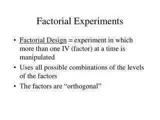
Factorial Treatments ( § 14.3, 14.4, 15.4). Completely randomized designs - One treatment factor at t levels. Randomized block design - One treatment factor at t levels, one block factor at b levels.

E N D
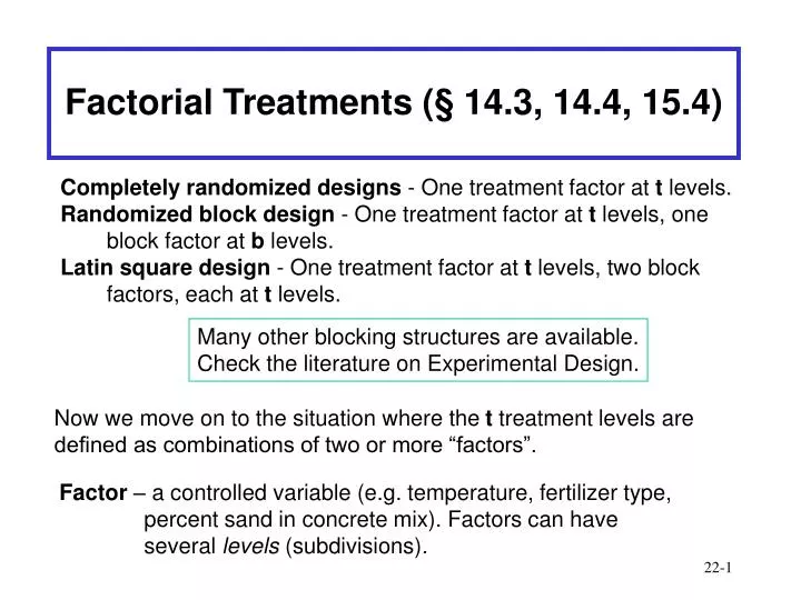
Factorial Treatments (§ 14.3, 14.4, 15.4) Completely randomized designs - One treatment factor att levels. Randomized block design - One treatment factor at t levels, one block factor at b levels. Latin square design - One treatment factor at tlevels, two block factors, each at t levels. Many other blocking structures are available. Check the literature on Experimental Design. Now we move on to the situation where the t treatment levels are defined as combinations of two or more “factors”. Factor – a controlled variable (e.g. temperature, fertilizer type, percent sand in concrete mix). Factors can have several levels (subdivisions).
Example 1 of Factors What factors (characteristics, conditions) will make a wiring harness for a car last longer? FACTOR Levels Number of strands 7 or 9. Length of unsoldered, 0, 3, 6, or 12. uninsulated wire (in 0.01 inches) Diameter of wire (gauge) 24, 22, or 20 A treatment is a specific combination of levels of the three factors. T1 = ( 7 strand, 0.06 in, 22 gauge) Response is the number of stress cycles the harness survives.
Example 2 of Factors What is the effect of temperature and pressure on the bonding strength of a new adhesive? Factor x1: temperature (any value between 30oF to 100oF) Factor x2: pressure (any value between 1 and 4 kg/cm2 Factors (temperature, pressure) have continuous levels, Treatments are combinations of factors at specific levels. Response is bonding strength - can be determined for any combination of the two factors. Response surface above the (x1 by x2) Cartesian surface.
Other Examples of Factors • The effect of added Nitrogen, Phosphorus and Potassium on crop yield. • The effect of replications and duration on added physical strength in weight lifting. • The effect of age and diet on weight loss achieved. • The effect of years of schooling and gender on Math scores. • The effect of a contaminant dose and body weight on liver enzyme levels. Since many of the responses we are interested in are affected by multiple factors, it is natural to think of treatments as being constructed as combinationsof factor levels.
One at a Time Approach Consider a Nitrogen and Phosphorus study on crop yield. Suppose two levels of each factor were chosen for study: N@(40,60), P@(10,20) lbs/acre. One-factor-at-a-time approach: Fix one factor then vary the other Treatment N P Yield Parameter T1 60 10 145 m1 T2 40 10 125 m2 T3 40 20 160 m3 H0: m1-m2 = test of N-effect (20 unit differenceobserved in response). H0: m2-m3 = test of P-effect (35 unit difference observed in response). If I examined the yield at N=60 and P=20 what would I expect to find? E(Y | N=60,P=20) = m3+(m1 - m2) =160 + 20 = 180? E(Y | N=60,P=20) = m2+(m1 - m2)+(m3 - m2) = 125+20+35 = 180?
Interaction and Parallel Lines We apply the N=60, P=20 treatment and get the following: Treatment N P Yield Parameter T1 60 10 145 m1 T2 40 10 125 m2 T3 40 20 160 m3 T4 60 20 130 m4 Yield Expected T4 180 170 T3 160 N=40 T1 150 140 Observed T4 N=60 20 130 T2 120 P 20 10
Parallel and Non-Parallel Profiles Parallel Lines => the effect of the two factors is additive (independent). Non-Parallel Lines => the effect of the two factors interacts (dependent). 180 170 160 N=40 150 140 N=60 20 130 120 P 20 10 The effect of one factor on the response does not remain the same for different levels of the second factor. That is, the factors do not act independently of each other. Without looking at all combinations of both factors, we would not be able to determine if the factors interact.
Factorial Experiment Factorial Experiment - an experiment in which the response y is observed at all factor level combinations. An experiment is not a design. (e.g. one can perform a factorial experiment in a completely randomized design, or in a randomized complete block design, or in a Latin square design.) Design relates to how the experimental units are arranged, grouped, selected and how treatments are allocated to units. Experiment relates to how the treatments are formed. In a factorial experiment, treatments are formed as combinations of factor levels. (E.g. a fractional factorial experiment uses only a fraction (1/2, 1/3, 1/4, etc.) of all possible factor level combinations.)
General Data Layout Two Factor (a x b) Factorial Column Factor (B) Row Factor(A) 1 2 3 … b Totals 1 T11 T12 T13 … T1b A1 2 T21 T22 T23 … T2b A2 3 T31 T32 T33 … T3b A3 … … … … … … ... a Ta1 Ta2 Ta3 … Tab Aa Totals B1 B2 B3 … Bb G yijk= observed response for the kth replicate (k=1,…,n) for the treatment defined by the combination of the ith level of the row factor and the jth level of the column factor.
Model mij = mean of the ijth table cell, expected value of the response for the combination for the ith row factor level and the jth column factor level. Overall Test of no treatment differences: Ho: all mij are equal Ha: at least two mij differ Test as in a completely randomized design with a x b treatments.
After the Overall F test • As with any experiment, if the hypothesis of equal cell means is rejected, the next step is to determine where the differences are. • In a factorial experiment, there are a number of predefined contrasts (linear comparisons) that are always of interest. • Main Effect of Treatment Factor A - Are there differences in the means of the factor A levels (averaged over the levels of factor B). • Main Effect of Treatment Factor B - Are there differences in the means of the factor B levels (averaged over the levels of factor A). • Interaction Effects of Factor A with Factor B - Are the differences between the levels of factor A the same for all levels of factor B? (or equivalently, are the differences among the levels of factor B the same for all levels of factor A? (Yes no interaction present; no interaction is present.)
Main Effects Column Factor (B) Row Factor(A) 1 2 3 … b 1 m11m12m13 … m1bm1 2 m21m22m13 … m1bm2 3 m31m32m13 … m1bm3 … … … … … … ... a ma1ma2ma3 … mabma Totals m1m2m3 … mbm Factor A main effects: Testing is via a set of linear comparisons.
Testing for Main Effects: Factor A There are a levels of Treatment Factor A. This implies that there are a-1 mutually independent linear contrasts that make up the test for main effects for Treatment Factor A. The Sums of Squares for the main effect for treatment differences among levels of Factor A is computed as the sum of the individual contrast sums of squares for any set of a-1 mutually independent linear comparisons of the a level means. Regardless of the chosen set, this overall main effect sums of squares will always equal the value of SSA below. Reject H0 if F > F(a-1),ab(n-1),a
Profile Analysis for Factor A Mean for level 5 of Factor A Mean for level 1 of Factor A m53 180 m11 m51 170 m5 160 m m1 150 m13 140 m52 m12 130 120 5 4 1 3 2 Factor A Levels Profile of mean of Factor A (main effect of A). Profile for level 2 of Factor B.
Insignificant Main Effect for Factor A m51 180 m11 170 m5 m13 160 m m1 150 140 m52 m12 130 120 5 4 1 3 2 Factor A Levels Is there strong evidence of a Main Effect for Factor A? SSA small (w.r.t. SSE) No.
Significant Main Effect for Factor A 180 170 160 m 150 140 130 120 5 4 1 3 2 Factor A Levels Is there strong evidence of a Main Effect for Factor A? SSA large (w.r.t. SSE) Yes.
Main Effect Linear Comparisons - Factor A Column Factor (B) Row Factor(A) 1 2 b=3 1 m11m12m13m1 2 m21m22m13m2 3 m31m32m13m3 4 m41m42m43m4 a=5 m51m52m53m5 Totals m1m2m3m Testing via a set of linear comparisons. Not mutually orthogonal, but together they represent a-1=4 dimensions of comparison.
Main Effect Linear Comparisons - Factor B Column Factor (B) Row Factor(A) 1 2 b=3 1 m11m12m13m1 2 m21m22m13m2 3 m31m32m13m3 4 m41m42m43m4 a=5 m51m52m53m5 Totals m1m2m3m Testing via a set of linear comparisons. Not mutually orthogonal, but together they represent b-1=2 dimensions of comparison.
Testing for Main Effects: Factor B There are b levels of Treatment Factor B. This implies that there are b-1 mutually independent linear contrasts that make up the test for main effects for Treatment Factor B. The Sums of Squares for the main effect for treatment differences among levels of Factor B is computed as the sum of the individual contrast sums of squares for any set of b-1 mutually independent linear comparisons of the b level means. Regardless of the chosen set, this overall main effect sums of squares will always equal the value of SSB below. Reject H0 if F > F(b-1),ab(n-1),a
Interaction Two Factors, A and B, are said to interact if the difference in mean response for two levels of one factor is not constant across levels of the second factor. 180 180 160 160 140 140 120 120 5 4 5 4 1 3 1 3 2 2 Factor A Levels Factor A Levels Differences between levels of Factor B donot depend on the level of Factor A. Differences between levels of Factor B do depend on the level of Factor A.
Interaction Linear Comparisons m51 m41 m21 180 m52 m31 Interaction is lack of consistency in differences between two levels of Factor B across levels of Factor A. m22 m42 m53 160 m11 m32 m43 140 m23 m12 m33 120 m13 5 4 1 3 2 Factor A Levels These four linear comparisons tested simultaneously is equivalent to testing that the profile line for level 1 of B is parallel to the profile line for level 2 of B. Four more similar contrasts would be needed to test the profile line for level 1 of B to that of level 3 of B.
Model for Interaction Tests for interaction are based on the abij terms exclusively. If allabijterms are equal to zero, then there is no interaction.
Overall Test for Interaction H0: No interaction, HA: Interaction exists. TS: F > F(a-1)(b-1),ab(n-1),a RR:
Partitioning of Total Sums of Squares TSS = SSR + SSE = SSA + SSB + SSAB + SSE ANOVA Table
Multiple Comparisons in Factorial Experiments • Methods are the same as in the one-way classification situation i.e. composition of yardstick. Just need to remember to use: • (i) MSE and df error from the SSE entry in AOV table; • (ii) n is the number of replicates that go into forming the sample means being compared; • (iii) t in Tukey’s HSD method is # of level means being compared. • Significant interactions can affect how multiple comparisons are performed. If Main Effects are significant AND Interactions are NOT significant: Use multiple comparisons on factor main effects (factor means). If Interactions ARE significant: 1) Multiple comparisons on main effect level means should NOT be done as they are meaningless. 2) Should instead perform multiple comparisons among all factorial means of interest.
Two Factor Factorial Example: pesticides and fruit trees (Example 14.6 in Ott & Longnecker, p.896) An experiment was conducted to determine the effect of 4 different pesticides (factor A) on the yield of fruit from 3 different varieties of a citrus tree (factor B). 8 trees from each variety were randomly selected; the 4 pesticides were applied to 2 trees of each variety. Yields (bushels/tree) obtained were: Pesticide (A) 1 2 3 4 Variety (B) 1 2 3 This is a completely randomized 3 4 factorial experiment with factor A at a=4 levels, and factor B at b=3 levels. There are t=34=12 treatments, each replicated n=2 times.
Stat > ANOVA > Two-way… AByield 1 1 49 1 1 39 1 2 55 1 2 41 1 3 66 1 3 68 2 1 50 2 1 55 2 2 67 2 2 58 2 3 85 2 3 92 3 1 43 3 1 38 3 2 53 3 2 42 3 3 69 3 3 62 4 1 53 4 1 48 4 2 85 4 2 73 4 3 85 4 3 99 Example in Minitab Two-way ANOVA: yield versus A, B Analysis of Variance for yield Source DF SS MS F P A 3 2227.5 742.5 17.56 0.000 B 2 3996.1 1998.0 47.24 0.000 Interaction 6 456.9 76.2 1.80 0.182 Error 12 507.5 42.3 Total 23 7188.0 Interaction not significant; refit additive model: Stat > ANOVA > Two-way > additive model Two-way ANOVA: yield versus A, B Source DF SS MS F P A 3 2227.46 742.49 13.86 0.000 B 2 3996.08 1998.04 37.29 0.000 Error 18 964.42 53.58 Total 23 7187.96 S = 7.320 R-Sq = 86.58% R-Sq(adj) = 82.86%
Analyze Main Effects with Tukey’s HSD (MTB) Stat > ANOVA > General Linear Model Use to get factor or profile plots MTB will use t=4 & n=6 to compare Amaineffects, and t=3 & n=8 to compare B main effects.
Tukey Analysis of Main Effects (MTB) A = 1 subtracted from: Difference SE of Adjusted A of Means Difference T-Value P-Value 2 14.833 4.226 3.5100 0.0122 3 -1.833 4.226 -0.4338 0.9719 4 20.833 4.226 4.9297 0.0006 A = 2 subtracted from: Difference SE of Adjusted A of Means Difference T-Value P-Value 3 -16.67 4.226 -3.944 0.0048 4 6.00 4.226 1.420 0.5038 A = 3 subtracted from: Difference SE of Adjusted A of Means Difference T-Value P-Value 4 22.67 4.226 5.364 0.0002 All Pairwise Comparisons among Levels of B B = 1 subtracted from: Difference SE of Adjusted B of Means Difference T-Value P-Value 2 12.38 3.660 3.381 0.0089 3 31.38 3.660 8.573 0.0000 B = 2 subtracted from: Difference SE of Adjusted B of Means Difference T-Value P-Value 3 19.00 3.660 5.191 0.0002 Summary: B1 B2 B3 Summary: A3 A1 A2 A4
Compare All Level Means with Tukey’s HSD (MTB) If the interaction had been significant, we would then compare all level means… MTB will use t=4*3=12& n=2 to compare all level combinations of A with B.
Tukey Comparison of All Level Means (MTB) A = 1, B = 1 subtracted from: Difference SE of Adjusted A B of Means Difference T-Value P-Value 1 2 4.000 6.503 0.6151 0.9999 1 3 23.000 6.503 3.5367 0.0983 2 1 8.500 6.503 1.3070 0.9623 2 2 18.500 6.503 2.8448 0.2695 2 3 44.500 6.503 6.8428 0.0007 3 1 -3.500 6.503 -0.5382 1.0000 3 2 3.500 6.503 0.5382 1.0000 3 3 21.500 6.503 3.3061 0.1395 4 1 6.500 6.503 0.9995 0.9945 4 2 35.000 6.503 5.3820 0.0055 4 3 48.000 6.503 7.3810 0.0003 ... etc. ... A = 4, B = 2 subtracted from: Difference SE of Adjusted A B of Means Difference T-Value P-Value 4 3 13.00 6.503 1.999 0.6882 There are a total of t(t-1)/2=12(11)/2=66 pairwise comparisons here! Note that if we wanted just the comparisons among levels of B (within each level of A), we should use t=3 & n=2. (Not possible in MTB.)
Example in R ANOVA Table: Model with interaction > fruit <- read.table("fruit.txt",header=T) > fruit.lm <- lm(yield~factor(A)+factor(B)+factor(A)*factor(B),data=fruit) > anova(fruit.lm) Df Sum Sq Mean Sq F value Pr(>F) factor(A) 3 2227.5 742.5 17.5563 0.0001098 *** factor(B) 2 3996.1 1998.0 47.2443 2.048e-06 *** factor(A):factor(B) 6 456.9 76.2 1.8007 0.1816844 Residuals 12 507.5 42.3 Main Effects: Interaction is not significant so fit additive model > summary(lm(yield~factor(A)+factor(B),data=fruit)) Call: lm(formula = yield ~ factor(A) + factor(B), data = fruit) Coefficients: Estimate Std. Error t value Pr(>|t|) (Intercept) 38.417 3.660 10.497 4.21e-09 *** factor(A)2 14.833 4.226 3.510 0.002501 ** factor(A)3 -1.833 4.226 -0.434 0.669577 factor(A)4 20.833 4.226 4.930 0.000108 *** factor(B)2 12.375 3.660 3.381 0.003327 ** factor(B)3 31.375 3.660 8.573 9.03e-08 ***
Profile Plot for the Example (R) Averaging the 2 reps, in each A,B combination gives a typical point on the graph: interaction.plot(fruit$A,fruit$B,fruit$yield) Level 3, Factor B Level 2, Factor B Level 1, Factor B
Pesticides and Fruit Trees Example in RCBD Layout Suppose now that the two replicates per treatment in the experiment were obtained at different locations (Farm 1, Farm 2). Pesticide (A) 1 2 3 4 Variety (B) 1 2 3 This is now a 3 4 factorial experiment in a randomized complete block design layout with factor A at 4 levels, factor B at 3 levels, and the location (block) factor at 2 levels. (There are still t=34=12 treatments.) The analysis would therefore proceed as in a 3-way ANOVA.