Download
1 / 95
950 likes | 963 Views
Motion Analysis. Mike Knowles mjk802@bham.ac.uk January 2006. Introduction. So far you have seen techniques for analysing static images – 2 Dimensional information Now we shall consider time-varying images – video. Variations in a scene through time are caused by motion. Motion.

E N D
Motion Analysis Mike Knowles mjk802@bham.ac.uk January 2006
Introduction • So far you have seen techniques for analysing static images – 2 Dimensional information • Now we shall consider time-varying images – video. • Variations in a scene through time are caused by motion
Motion • Motion analysis allows us to extract much useful information from a scene: • Object locations and tracks • Camera Motion • 3D Geometry of the scene
Contents • Perspective and motion geometry • Optical flow • Estimation of flow • Feature point detection, matching and tracking • Techniques for tracking moving objects • Structure from motion
Perspective Geometry • An image can be modelled as a projection of the scene at a distance of f from the optical centre O • Note convention: capital letters denote scene properties, lowercase for image properties
Perspective Geometry • The position of our point in the image is related to the position in 3D space by the perspective projection:
Motion Geometry • If the point is moving in space then it will also move in the image • Thus we have a set if vectors v(x,y) describing the motion present in the image at a given position – This is the Optical flow
Optical Flow • An optical flow field is simply a set of vectors describing the image motion at any point in the image.
Estimating Optical Flow • In order to estimate optical flow we need to study adjacent frame pairs • There are 2 approaches we can take to this: • Greylevel gradient based methods • ‘Interesting’ feature matching
Greylevel conservation • If we have a perfect optical flow field:
Greylevel conservation • Generally we measure time in frames so dt = 1 • This leaves us with
Greylevel Conservation • Taking a Taylor expansion and eliminating the higher order terms:
Greylevel Conservation • Tidying up we are left with: • This is the standard form of the greylevel constraint equation • But…..
Limitations of the greylevel constraint equation • The greylevel constraint equation only allows us to measure the flow in the direction of the greylevel image gradient
The aperture problem • Consider a plot in (vx , vy) space, at a single point in space - the greylevel conservation equation gives a line on which the true flow lies
The aperture problem • Thus we cannot generate a flow vector for a single point – we have to use a window • The larger the window is the better the chance of overcoming this problem • But the larger the window the greater the chance of the motion being different • This is called the aperture problem
Overcoming the aperture problem • Several solutions have been proposed: • Assume v(x,y) is smooth (Horn and Schunck’s algorithm) • Assume v(x,y) is locally piecewise linear or constant (Lucas and Kanade’s algorithm) • Assume v(x,y) obeys some simple model (Black and Annandan’s algorithm) • We shall consider the latter two solutions
Assuming a locally constant field • This algorithm assumes that the flow field around some point is constant
The model • Model: • This model is valid for points in some -point neighbourhood where the optical flow is assumed constant.
Noise • n(x,y,t) is noise corrupting the true greylevel values and is assumed zero-mean and uncorrelated with variance:
We can linearise our model: • Where:
For each point we have an equation: • We can write this in matrix form:
We can solve for using a least squares technique: • The result is:
We are also interested in the quality of the estimate as measured by the covariance matrix of: • It can be shown that: • Thus we can determine the variances of the estimates of the components vx and vy
We can use the covariance matrix to determine a confidence ellipse at a certain probability (e.g. 99%) that the flow lies in that ellipse
It can be seen from the expression for the variance estimates that the accuracy of the algorithm depends on: • Noise variance • Size of the neighbourhood • Edge business
Modelling Flow • An alternative to assuming constant flow is to use a model of the flow field • One such model is the Affine model:
Estimating motion models • Black and Annandan propose an algorithm for estimating the parameters of the the model parameters • This uses robust estimation to separate different classes of motion
Minimisation of Error Function • Once again, if we are to find the optimum parameters we need an error function to minimise: • But this is not in a form that is easy to minimise…
Gradient-based Formulation • Applying Taylor expansion to the error function: • This is the greylevel constraint equation again
Gradient-descent Minimisation • If we know how the error changes with respect to the parameters, we can home in on the minimum error
Applying Gradient Descent • We need: • Using the chain rule:
Robust Estimation • What about points that do not belong to the motion we are estimating? • These will pull the solution away from the true one
Robust Estimators • Robust estimators decrease the effect of outliers on estimation
Error w.r.t. parameters • The complete function is:
Aside – Influence Function • It can be seen that the first derivative of the robust estimator is used in the minimisation:
Pyramid Approach • Trying to estimate the parameters form scratch at full scale can be wasteful • Therefore a ‘pyramid of resolutions’ or ‘Gaussian pyramid’ is used • The principle is to estimate the parameters on a smaller scale and refine until full scale is reached
Pyramid of Resolutions • Each level in the pyramid is half the scale of the one below – i.e. a quarter of the area
Out pops the solution…. • When combined with a suitable gradient based minimisation scheme… • Black and Annadan suggest the use of Graduated Non-convexity
Feature Matching • Feature point matching offers an alternative to gradient based techniques for finding optical flow • The principle is to extract the locations of particular features from the frame and track their position in subsequent frames
Feature point selection • Feature points must be : • Local (extended line segments are no good, we require local disparity) • Distinct (a lot ‘different’ from neighbouring points) • Invariant (to rotation, scale, illumination) • The matching process must be : • Local (thus limiting the search area) • Consistent (leading to ‘smooth’ disparity estimates)
Approaches to Feature point selection • Previous approaches to feature point selection have been • Moravec interest operator, this is based on thresholding local greylevel squared differences • Symmetric features e.g. circular features, spirals • Line segment endpoints • Corner points
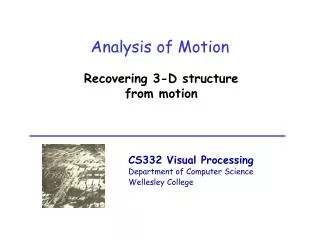
Motion and 3D Structure From Optical Flow • This area of computer vision attempts to reconstruct the structure of the 3D environment and the motion of objects within it using optical flow • Applications are many, the dominant one is autonomous navigation
As we saw previously, the relationship between image plane motion and the 3D motion that it describes is summed up by the perspective projection
The perspective projection is described as: • We can differentiate this w.r.t. time:
Substituting in the original perspective projection equation: • We can invert this by solving for
This gives us two components – one parallel to the image plane and one along our line of sight