Benchmark dataset processing

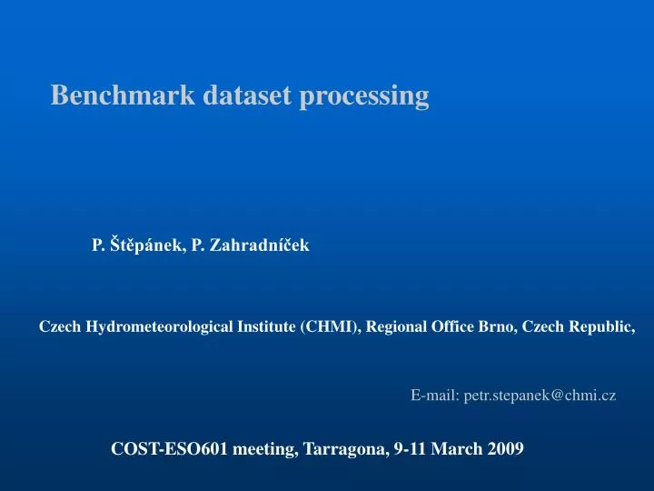
1. Benchmark dataset processing P. Štěpánek, P. Zahradníček Czech Hydrometeorological Institute (CHMI), Regional Office Brno, Czech Republic, E-mail: petr.stepanek@chmi.cz COST-ESO601 meeting, Tarragona, 9-11 March 2009

2. Outline • Outliers (daily data) • Detection (monthly data) + correction (daily data) (description of methodology) • Benchmark dataset (monthly data)

3. Processing before any data analysis Software AnClim, ProClimDB

4. Data Quality Control Finding Outliers Two main approaches: • Using limits derived from interquartile ranges(time series) • comparing values to values of neighbouring stations(spatial analysis)

5. Example of outputs for outliers assessment Suspicious values Expected value Neighbour stations values Altitudes and distances of neighbours List of neighbours

6. Quality control Spatial distribution • Run for period 1961-2007, daily data (measured values in observation hours) • All stations (200 climatological stations, 800 precipitation stations) • All meteorological elements (T, TMA, TMI, TPM, SRA, SCE, SNO, E, RV, H, F) – parameters set individually • Historical records will follow now

7. Air temperature, number of outliers 1961-2007, from 3.431.000 station-days T – air temperature at obs. hour, TMA – daily maximum temp., TMI – daily min. temp., TPM – daily ground minimum temp.

8. Air temperature, number of outliers 1961-2007, from 3.431.000 station-days Air temperature at obs. hour, AVG – daily average temp.

9. Air temperature, number of outliers 1961-2007, from 3.431.000 station-days TMA – daily maximum temp., TMI – daily min. temp., TPM – daily ground minimum temp.

10. Air temperature, number of outliers 1961-2007, Number of outliers per one station(all observation hours, AVG)

11. Spatial distribution of precipitation stations Spatial distribution • period 1961-2007 • 600 stations • mean minimum distance: 7.5 km

12. Problematic detections (heavy rainfall)

13. Problematic detections (heavy rainfall), Radar information

14. Precipitation, number of outliers 1961-2007, from 13.724.000station-days .

15. Precipitation, number of outliers 1961-2007, Number of outliers per one station

16. Conclusions • Only combination of several methods for outliers detection leads to satisfying results (“real” outliers detection, supressing fault detection -> Emsemble approach) • Parameters (settings) has to be found individually for each meteorological element, maybe also region (terrain complexity) and part of a year (noticeable annual cycle in number of outliers) • Similar to homogenization of time series, it is important to use measured value (e.g. from observation hours) - outliers are masked in daily average (and even more in monthly or annual ones) • Errors found in all elements and investigated countries(AT, CZ, SK, HU)

17. Experiences with homogenization in the Czech Republic

18. Homogenization • Change of measuring conditions inhomogeneities

19. DetectingInhomogeneities by SNHT (p=0.05, 950 series) Detection A

20. we depend upon statistical tests results Assessing Homogeneity - Problems • most of metadata incomplete • uncertainty in test results - right inhomogeneity detection is problematic (for smaller amount of change)

21. „Ensemble“ approach - processing of big amount of test resultsfor each individual series Proposed solution SOLUTION • most of metadata incomplete • uncertainty in test results - the right inhomogeneity detection is problematic • To get as many test results for each candidate series as possible • For each year, group of years and whole series: portion of number of detected inhomogenities in number of all possible (theoretical) detections

22. How to increase number of test results Diagram Days, Months, seasons, year

23. Creating Reference Series • for monthly, daily data (each month individually) • weighted/unweighted mean from neighbouring stations • criterions used for stations selection (or combination of it): • best correlated / nearest neighbours (correlations – from the first differenced series) • limit correlation, limit distance • limit difference in altitudes • neighbouring stations series should be standardized to test series AVG and / or STD (temperature - elevation, precipitation - variance) - missing data are not so big problem then

24. Relative homogeneity testing • Available tests: • Alexandersson SNHT • Bivariate test of Maronna and Yohai • Mann – Whitney – Pettit test • t-test • Easterling and Peterson test • Vincent method • … 20 year parts of the daily series(40 for monthly series with 10 years overlap), in SNHT splitting into subperiods in position of detected significant changepoint (30-40 years per one inhomogeneity)

25. Homogeneity assessment Homogeneity assessment Output example: Station Čáslav, 3rd segment, 1911-1950, n=40 • Quality control • Homogenization • Data Analysis

26. Homogeneity assessment, Output II example: Homogeneity assessment Summed numbers of detections for individual years

27. Homogeneity assessment Homogeneity assessment • combining several outputs (sums of detections in individual years, metadata, graphs of differences/ratios, …)

28. Adjusting monthly data • using reference series based on correlations • adjustment: from differences/ratios 20 years before and after a change, monhtly • smoothing monthly adjustments (low-pass filter for adjacent values)

29. Example: Adjusting values - evaluation Example combining series

30. Iterative homogeneity testing • several iteration of testing and results evaluation • several iterations of homogeneity testing and series adjusting (3 iterations should be sufficient) • question of homogeneity of reference series is thus solved: • possible inhomogeneities should be eliminated by using averages of several neighbouring stations • if this is not true: in next iteration neighbours should be already homogenized

31. Dependence of tested series on reference series Filling missing values • Before homogenization: influence on right inhomogeneity detection • After homogenization: more precise - data are not influenced by possible shifts in the series

32. Homogenization of the series in the Czech Republic

33. Correlations between tested and reference series Air temperature Graphs - selection Boxplots: - Median - Upper and lower quartiles (for 200 testes series)

34. Correlations between tested and reference series Precipitation, snow depth, new snow Graphs - selection Boxplots: - Median - Upper and lower quartiles (for 800 testes series)

35. Correlations between tested and reference series Wind speed Graphs - selection Boxplots: - Median - Upper and lower quartiles (for 200 testes series)

36. Homogeneity testing resultsAir temperature Number of significant inhomogeneities (0.05) detected by used tests (A, B tests, c and d reference series, alltogether)

37. Homogeneity testing resultsAir temperature Amount of adjustments, averages of absolute values, T_AVG

38. Homogeneity testing resultsPrecipitation • 4 tests, 4 reference series, 12 months + 4 seasons and year • Number of detected inhomogeneities (significant)

39. Amount of change (ratios – standardized to be >1.0), precipitation (reference series calculation based on correlations) Graphs - adjsust Boxplots: - Median - Upper and lower quartiles (for 589 testes series) Correlation improvement

40. HomogenizationFinal remarks, recommendations 1/2 • data quality control before homogenization is of very importance (if it is not part of it) • Using series of observation hours (complementarily to daily AVG) is highly recommended(different manifestation of breaks) • be aware of annual cycle of inhomogeneities, adjustments, … • to know behavior of spatial correlations (of element being processed) to be able to create reference series of sufficient quality …

41. HomogenizationFinal remarks, recommendations 2/2 • Because of Noise in the time seriesit makes sense: • - „Ensemble“ approach to homogenization (combining information from different statistical tests, time frames, overlapping periods, reference series, meteorological elements, …) • - more information for inhomogeneities assessment – higher quality of homogenization in case metadata are incomplete

42. Software used for data processing • LoadData - application for downloading data from central database (e.g. Oracle) • ProClimDB software for processing whole dataset (finding outliers, combining series, creating reference series, preparing data for homogeneity testing, extreme value analysis, RCM outputs validation, correction, …) • AnClim software for homogeneity testing http://www.climahom.eu

43. AnClim software AnClim software

44. ProClimDB software ProcData software

45. Testing of benchmark dataset • Fully automated (just for one click), but it should not work like this in reality: detection phase can be fully automated, but desicion about breaks to be corrected should be man-made (comparison with metadata, plots of differences – ratios, …)

46. Fully automatic detection phase in ProClimDB softwareselecting neighbours for reference series

47. Fully automatic detection phase in ProClimDB softwarereference series calculation and launching AnClim

48. Automation in AnClim, tests can be selected in advance

49. Test results processed back in ProClimDB

50. Non-automated desicion about breaks before correction