Download

1 / 30
300 likes | 306 Views
Spotted Microarray Workshop. Microarray Data Preprocessing and Clustering Analysis. Liangjiang (LJ) Wang ljwang@ksu.edu KSU Bioinformatics Center, Biology Division June, 2005. Outline. Overview of microarray data analysis. Microarray data preprocessing.

E N D
Spotted Microarray Workshop Microarray Data Preprocessing and Clustering Analysis Liangjiang (LJ) Wang ljwang@ksu.edu KSU Bioinformatics Center, Biology Division June, 2005
Outline • Overview of microarray data analysis. • Microarray data preprocessing. • Statistical inference of significant genes. • Clustering analysis and visualization. • Microarray databases and standards.
Spotted Microarray Reference Cells Experimental Cells Samples Gene expression matrix (ratios) Extract mRNA Genes Make and label cDNA Array image data Hybridize Probes
Overview of Microarray Data Analysis Microarray experiment Image analysis and data normalization Sample classification Statistical inference of significant genes Clustering analysis of co-expressed genes List of significant or co-expressed genes Promoter analysis, gene function prediction, and pathway analysis
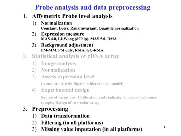
Microarray Image Analysis • Spot finding: place a grid to identify spot locations. • Segmentation: separate each spot (foreground) from the background. • Spot intensity extraction: often use mean or median intensity of all the pixels within a spot. • Background subtraction: may subtract local background or globally estimated background.
Microarray Data Normalization • To remove the systemic bias in the data so that meaningful biological comparisons can be made: • Unequal quantities of starting RNA. • Differences in labeling (e.g., Cy3 versus Cy5). • Different detection efficiencies between the dyes. • Differences in hybridization and washing. • Other experimental variations. • Normalization is based on some assumptions: • A subset of genes (housekeeping genes) is assumed to be constant. • The total intensity or overall intensity distributions between the two channels are comparable.
Global Normalization • Total intensity normalization: • A normalization factor is calculated by summing the measured intensities in both channels and then taking the ratio: • All the intensities in one channel are multiplied by the normalization factor: • A subset of genes (housekeeping genes) may be also used for the global normalization.
Scatter Plot of Cy3 vs Cy5 Intensities Intensities from “self-self” hybridization After normalization Before normalization (Quackenbush, 2001)
(Quackenbush, 2001) (Quackenbush, 2001) Raw data After lowess 0 log ratio, log2(R/G) log ratio, log2(R/G) 0 Lowess Normalization • Probably the most widely used approach for spotted microarray normalization. • A locally weighted linear repression is used to estimate the systematic bias in the data. Ratio-Intensity (R-I) plot (also called MA plot)
Why Log Transformation? • Log2(R/G) treats up-regulated and down-regulated genes in a similar fashion: • If R/G = 4, log2(R/G) = 2. • If R/G = 1/4 = 0.25, log2(1/4) = -2. • Log normalizes distribution.
Finding Significant Genes • Fold change: uses a single fold change threshold to select genes; does not take into account the biological and experimental variability. • Statistical tests: t test, SAM and ANOVA; require a number of replicates for each condition.
Statistical significance → high (Wolfinger et al., 2001) Volcano Plot Larger fold changes does not necessarily mean higher significance levels.
Student’s t Test • To test whether there is a significant difference in gene expression measurements between two conditions (A and B): • H0: no difference in gene expression, • H1: the gene is differentially expressed, • Test statistic: • Calculate the probability (p value) of the t statistic with degree of freedom, df = nA + nB - 2. • Assume a 95% confidence level (i.e., 5% falsepositive rate).If p≤ 0.05, reject the null hypothesis.
Problem of Multiple Testing Suppose that you have 5,000 genes on your microarray, and you select the genes with p≤ 0.05 (i.e., 5% false positive rate). Because you have applied 5,000 times of the t test, you may have 5,000 x 0.05 = 250 false positives!
Correction for Multiple Testing • Bonferroni correction: • Set the significance cutoff, p' = α/N, where α is the false positive rate, and N is the number of genes. • For example, if you have 5,000 genes in your microarray, and you expect 5% of false positives, the significance cutoff, p' = 0.05/5000 = 1.0E-5. • False Discovery Rate (FDR): • Rank all the genes by significance (p value) so that the top gene has the most significant p value. • Start from the top of the list, and accept the genes if i: the rank of the gene in the list. N: the number of genes in the array. q: the desired FDR.
SAM Plot Up-regulated Observed d = expected d Significance cutoffs Observed d statistic Down-regulated Expected d statistic SAM: Significance Analysis of Microarrays • SAM (http://www-stat.stanford.edu/~tibs/SAM/) is a modified t test. • The observed d statistic is computed from the data, and the expected d statistic is assessed by permutation. • With a user-defined FDR, SAM derives the significance cutoffs for selecting up- and down-regulated genes.
ANOVA • ANalysis Of VAriance (ANOVA) is used to find significant genes in more than two conditions: • For each gene, compute the F statistic. • Calculate the p value for the F statistic. • Adjust the significance cutoff for multiple testing.
Clustering Analysis • Clustering analysis is to partition a dataset into a few groups (clusters) such that: • Homogeneity: objects in the same cluster are similar to each other. • Separation: dissimilar objects are placed in different clusters. • In microarray data analysis, this • means to find groups of genes (or samples) with similar gene expression patterns. • Two key questions: • How to measure similarity of gene expression? • How to find these gene clusters?
B b2 d A a2 Sample 2 α a1 b1 Sample 1 Distance Metrics • Expression vector: each gene can be represented as a vector in the N-dimensional • hyperspace, where N is the • number of samples. • Euclidean distance: • Vector angle: • Pearson correlation coefficient:
— Gene A — Gene B — Gene A — Gene B Log(ratio) Z score dAB = 3.58 dAB = 0.36 Samples Samples Z Transformation • If Euclidean distance is used for clustering analysis, z transformation of the gene expression matrix may be necessary. • For each gene, calculate the z scores of the expression values:
a b c d e Step 1 Step 2 Step 3 Step 4 Step 0 Hierarchical Clustering Initialization:each object is a cluster Iteration Merge two clusters which are most similar to each other Until all objects are merged into a single cluster a b a b c d e c d e d e Agglomerative approach
CL SL AL Hierarchical Clustering (Cont’d) • Calculating distances between clusters: • Single linkage: takes the shortest distance between two clusters. • Complete linkage: uses the largest distance between two clusters. • Average linkage: uses the average distance between two clusters. • The clustering results are visualized using a tree (called dendrogram) with color-coded gene expression levels. • Hierarchical clustering can be applied to genes, samples, or both.
Sample Clustering Alizadeh, et al., 2000. Distinct types of diffuse large B-cell lymphoma identified by gene expression profiling. Nature, 403:503-511.
k = 2 k-Means Clustering Initialization User-defined k (# clusters) Randomly place k vectors (called centroids) in the data space Iteration Each object is assigned to its closest centroid Re-compute each centroid by taking the mean of data vectors currently assigned to the cluster Until the cluster centroids no longer change Iteration 0: 1: 2: 3:
Self-Organizing Map (SOM) • The user defines an initial geometry of nodes (reference vectors) for the partitions such as a 3 x 2 rectangular grid. • During the iterative “training” process, the nodes migrate to fit the gene expression data. • The genes are mapped to the most similar reference vector.
Clustering analysis of a yeast cell cycle time-series dataset k-means SOM 237 genes 194 genes
Tools for Microarray Data Analysis • GenePix (http://www.axon.com/GN_GenePixSoftware.html): commercial software for microarray image analysis. • GeneSpring (http://www.silicongenetics.com/cgi/SiG.cgi/Products/GeneSpring/index.smf): commercial software for microarray data analysis. • TIGR MeV (http://www.tm4.org/mev.html): free software for clustering, visualization, classification and statistical analysis of microarray data. • Bioconductor (http://www.bioconductor.org/): open source, free software for the analysis of genomic data. For microarray data analysis, most of the statistical methods are implemented in R.
Microarray Databases • Gene Expression Omnibus (GEO) at NCBI (http://www.ncbi.nlm.nih.gov/geo/): a public repository for high throughput gene expression data. • ArrayExpress at EBI (http://www.ebi.ac.uk/arrayexpress/): a public repository for microarray gene expression data; MIAME compliant. • Stanford Microarray Database (SMD at http://genome-www5.stanford.edu/): stores raw and normalized microarray data; provides data retrieval and online data processing.
The MIAME Standard • MIAME (Minimum Information About a Microarray Experiment) is a microarray data standard proposed by the Microarray Gene Expression Database group (MGED, http://www.mged.org/). • MIAME (http://www.mged.org/Workgroups/MIAME/) is needed to interpret the results from a microarray experiment and potentially to reproduce the microarray experiment. • MIAME checklist helps authors, reviewers and editors of scientific journals to meet the MIAME requirements and to make microarray data available to the community in a useful way.
Summary • Image analysis and data normalization are important preprocessing steps for microarray data analysis. • Statistical methods are available for selecting significantly up- or down-regulated genes. • Clustering analysis is widely used to explore and visualize microarray data. • The resulting significant or co-expressed genes can be further investigated using Gene Ontology annotation and promoter analysis.