Download
1 / 29
290 likes | 296 Views
In this study, we investigate the problem of retarded potentials in electromagnetism, similar to the force of attraction between the Earth and the Sun. We calculate the expected electric field using the Lienard-Weichert formula for an electrical charge with constant velocity. Experimental measurements are compared to theoretical calculations, showing the need for further understanding of the Coulomb field.

E N D
Measuring Propagation Speed of Coulomb Fields R. de Sangro, G. Finocchiaro, P.Patteri, M. Piccolo, G. Pizzella Eur. Phys. J. C (2015) 75-137
The force attracting the Earth to the Sun is directed to a point where the Sun actually is, not to the point where we see it We study now the problem in electromagnetism, where a similar situation occurs
Let us calculate the electric field expected when using the L-W formula
Measuring Emax Detector At y=30 cm at g=1000
The experiment at BTF (measurements made from 2009 thru 2014) beam length L = 3 m
Normalized amplitudes Sn for sensors A1(upper) and A3(lower)for A5;A6 =172.0 cm. The continuous line at 8.98+-0.54 mV (upper) and10.25+-0.59 mV (lower) indicate the weighted average of our measurements.The six measurements plotted refers to the transverse positions of A5, A6. The dashed line:
Upper graph: the ratio Vmax(A5)/Vmax(A1) at A5;A6=172.0 cmversus the transverse distance. Lower graph: Vmax(A6)/Vmax(A3) . The continuous lines are the theoretical ones
In spite of the very good agreement between measurements and calculations, we want to make sure that we do measure the Coulomb field and not measure electromagnetic radiation. • We put a lead block between the reference sensors A1,A2,A3,A4 and the movable sensors A5, A6, in order to stop the beam and forbid it to go under the sensors A5,A6.
conclusion Assuming that the electric field of the electron beams act on our sensor only after the beam itself has exited the beam pipe, the L.W model predicts sensors responses orders of magnitudes smaller than what we measure. The Feynman interpretation of the Lienard-Weichert formula for uniformly moving charges does not show consistency with our experimental data. Even if the steady state charge motion in our experiment lasted few tens of nanoseconds, our measurements indicate that everything behaves as if this state lasted for much longer.