Download
1 / 26
260 likes | 452 Views
Counter-current flows in liquid-liquid boundary layers II. Mass transfer kinetics. E. Horvath 1 , E. Nagy 1 , Chr. Boyadjiev 2 , J. Gyenis 1 1 University of Veszprém, Research Institute Chemical Process Engineering, 8201 Veszprém , P.O.B. 125, Hungary

E N D
Counter-current flows in liquid-liquid boundary layersII. Mass transfer kinetics E. Horvath1 , E. Nagy1 , Chr. Boyadjiev2 , J. Gyenis1 1 University of Veszprém, Research Institute Chemical Process Engineering,8201 Veszprém, P.O.B. 125, Hungary 2 Bulgarian Academy of Sciences , Institute of Chemical Engineering,1113 Sofia , Bl. 103 , Bulgaria Contents Abstract 1. Introduction2. Mathematical model 3. Method of solution 4. Numerical results 5. Mass transfer kinetics 6. Comparison between counter-current and co-current flows 7. Conclusion
Abstract A theoretical analysis of mass transfer kinetics based on similarity variables method for liquid-liquid counter - current flow has been done. The obtained numerical results for the mass transfer rate (Sherwood number) in case of a laminar boundary layer with flat phase boundary are compared with analogous results for co - current flow. The ratio between the mass transfer velocity and the dissipation energy in boundary layer is determined. The advantages of co-current flow because of lower energy losses than in case of counter-current one are shown. 1. Introduction In the first part of the work the velocity distribution in a laminar boundary layer of liquid - liquid counter - current flow with flat phase boundary was determined. They allowed the determination of dissipation energy at the boundary layer and its comparison with the one in case of co - current flow. The subject of the present work is the influence on the mass transfer kinetics caused by significant difference in the velocity profiles in laminar boundary layer in case of co - and counter-current flows. In this work the concentration distribution in a laminar boundary layer of liquid-liquid counter-current flow with flat phase boundary was determined. A theoretical analysis of mass transfer kinetics based on similarity variables method for liquid-liquid counter-current flow has been done.
2. Mathematical model The mass transfer rate is determined by the solution of the convection-diffusion equation. Boundary conditions at the phase boundary are introduced for the case of mass transfer between liquid and liquid to take into account the existence of thermodynamically equilibrium and the continuity of mass flux. In this way, the mathematical model of the interphase mass transfer in liquid-liquid systems with counter-current flow in a laminar boundary layer with flat phase boundary takes the following form: ; ; , i=1,2; boundary conditions: x = 0 , y ≥ 0 , c1 = c2∞ , u1 = u1∞; x = l , y ≤ 0 , c2 = c2∞ , u2 = - u2∞; y → ∞ , 0 ≤ x ≤ l , c1 = c1∞ , u1 = u1∞; y → - ∞ , 0 ≤ x ≤ l , c2 = c2∞ , u2 = - u2∞; y = 0 , 0 < x < l , u1 = u2 , v1 = v2 = 0 , c1 = χ c2 , , . Where ui and vi(i=1,2) are the velocity components in the liquid, and ci∞ (i=1,2) are the input concentrations of the absorbed substance.
3. Method of solution The problem can be presented in almost dimensionless form using two different coordinate systems for the two phases, so that the flow in each phase is oriented to the longitudinal coordinate. The following dimensionless variables and parameters are introduced. Dimensionless variables: ; ; ; , , ; , , ; Dimensionless parameters: , , i=1,2, , , , i=1,2, , ,
In the new coordinate systems , the model of counter - current flows has the following form: , , , ; , , i=1,2. , boundary conditions: , , , , , , , , , , , , i=1,2. The solution of the differential equation system should be made after the introduction of following similarity variables: Similarity variables: , i=1,2 , , i=1,2 , , , , i=1,2 .
Substitution of the similarity variables into the almost dimensionless mathematical model leads to: , , i=1,2 ; Boundary conditions: , , i=1,2 , , , , , , , , i=1,2 . The boundary conditions a and b were determined in previous work. It is clearly seen that it is possible to obtain the similarity solution for different values of X1=1–X2. For this purpose, values of X1 within the interval (0,1) are taken. The system is investigated at θ1 = 0.7, θ2 = 1.2, Sc1=812, Sc1=440 and θ3 = 0.8029. The solution of this common differential equations systems will be obtained at new boundary conditions for φi (i=1,2): , , , , where α and β are determined for different values of X1 so that the conditions , (i=1,2)are fulfilled.
4. Numerical results The numerical results could be obtained for interphase mass transfer of the liquid with middle solubility, the diffusion resistances are commensurable . The system which was modelling at 20 °C has mass transfer of acetic acid between water (1. phase) and tetra-chlorine-methane (2. phase) on the interface of contact of the two phases. The common differential equations system obtained should be solved after the introduction of boundary conditions for different values of X1. The numerical results show that the thicknesses of diffusion boundary layers (concentration distribution layers) is much less than laminar boundary layers’ thickness (velocity distribution layers). When the concentration boundary layer line is between contact interface of the two phases and zero velocity line where the velocity is equal to zero i.e. the velocity changes its direction in the phase, different dimensionless form of the convection-diffusion equation should have been used, because then the velocity did not change its direction in the concentration boundary layers. Therefore the length of the system should have been divided into 3 parts. One of them is then (0 < X1 < X0) the zero velocity line is above the concentration boundary layer lines, other one is then (X1≈ X0) we are in environment of the point where the velocity zero line cuts the X-coordinate and the third one is then (X0 < X1 < 1) the zero velocity line is below the concentration boundary layers lines. By reason of them the different convection-diffusion equations have the following forms in the three areas: 0 < X1 < X0 , ξ = I , X1 = X0 , ξ = i + 1 , X0 < X1 < 1 , ξ = 0 . where:
Zero velocity line and the velocity distribution from numerical results at θ1 = 0.7 and θ2 = 1.2 . Numerical results for the calculated values of the boundary conditions (α, β), the dimensionless mass flux at the interface ( φ′1(0), φ′2(0) ) and the boundary layers thicknesses (ηi∞, i=1,2), where φi(ηi∞) ≤0.01, are shown in the table. Dimensionless concentration distributions in the phases can be seen in the figures. Numerical results at values of θ1 = 0.7 , θ2 = 1.2, θ3 = 0.8029, X1=0.1.
Numerical results at values of θ1 = 0.7 , θ2 = 1.2, θ3 = 0.8029, X1=0.5902. Numerical results at values of θ1 = 0.7 , θ2 = 1.2, θ3 = 0.8029, X1=0.9.
5. Mass transfer kinetics The mass transfer rate may be expressed by the mass transfer coefficient and the average diffusion flux along the length of the phase boundary: , i=1,2 , which allows us to further determine the Sherwood number , i=1,2 . This equation can be presented by following form using the dimensionless variables, parameters and similarity variables: , , i=1,2 .
6. Comparison between counter-current and co-current flows The obtained solution of common differential equation system with boundary conditions gives the possibility for determination of mass transfer velocity rate using the average diffusion flux: , i=1,2. The average mass flux values for the system in case of counter current flows are shown in the following table. For purpose of comparison between the counter-current flow mass transfer velocity rate and co-current one, the common differential equation system should be solved using parameter’s values corresponding to co-current flow. These parameter’s values are shown in the head of the following table having asterisk sign. In case of co-current flow doesn’t depend on X1 so the mass transfer velocity rate can be presented in the following form: Ji* = –2φ′i(0). The obtained results are shown also in the following table.
The comparison of these results show that the counter - current flow mass transfer rate is much higher than in case of co - current flow in the phase 2. But it can’t be established in the phase 1, because these are almost equal. The obtained results in both parts of work allow us to determine the ratio between the mass transfer rate and the corresponding dissipation energy in case of counter - current and co - current flows: . , Comparative data for mass transfer energy efficiency (Ai , i = 1,2) in case of counter - current and co - current liquid - liquid flows are presented . The data show higher efficiency of co - current flow that is higher mass transfer velocity rate at equal energy losses. 7. Conclusion The obtained numerical results for the mass transfer between liquid - liquid counter - current flow show that the interface mass transfer rate (Ji , i = 1,2) is limited by the diffusion resistance of the phase 2 for small values of X1, i.e. J = J2. Otherwise when X1 is big the diffusion resistances are commensurable in the phases. In counter - current flows the velocity does not change its direction in the concentration boundary layers near the interface . The velocity changes its direction in the phases at different X1 (0 < X1 < X0 in the phase 1 , X0 < X1 < 1 in the phase 2) . The obtained results show that the co - current flow is more efficient energetically than the counter - current one because of the lower energy losses at equal rates of the mass transfer .