Download
1 / 40
520 likes | 768 Views
Seismic Tomography without Earthquakes: Progress in Ambient Noise Tomography. Mike Ritzwoller 1 Ying Yang 1 Morgan Moschetti 1 Fan-Chi Lin 1 Greg Bensen 1 Xiaodong Song 2 Sihua Zheng 3 1 - University of Colorado at Boulder 2 - University of Illinois, Urbana-Champaign

E N D
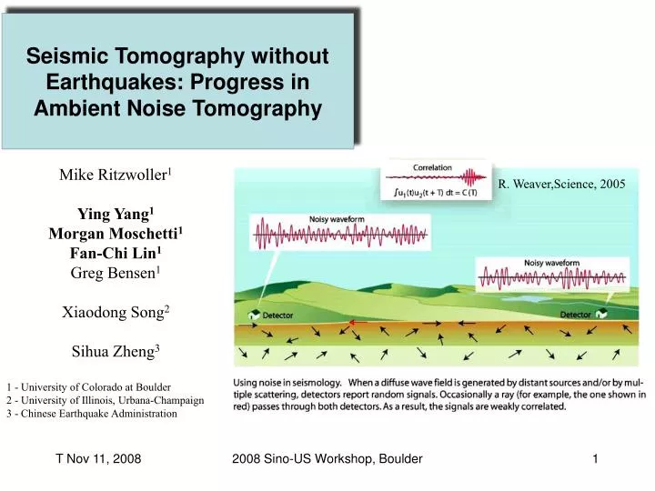
Seismic Tomography without Earthquakes: Progress in Ambient Noise Tomography Mike Ritzwoller1 Ying Yang1 Morgan Moschetti1 Fan-Chi Lin1 Greg Bensen1 Xiaodong Song2 Sihua Zheng3 1 - University of Colorado at Boulder 2 - University of Illinois, Urbana-Champaign 3 - Chinese Earthquake Administration R. Weaver,Science, 2005 2008 Sino-US Workshop, Boulder
Why Ambient Noise Tomography? • Ambient noise is enriched at short periods: 5 – 25 sec. Better constraints on crustal and uppermost mantle structure than information from earthquakes. • Particularly useful in aseismic areas; e.g., continental interiors. • For temporary deployments -- do not have to wait for earthquakes to occur. • Measurements are repeatable: rigorous uncertainty estimates. 2008 Sino-US Workshop, Boulder
Outline • Why do we believe results from ANT? 2. Application to the EarthScope Transportable Array (TA) across the western US: Isotropic and radially anisotropic 3D model in W. US. 3. New method of tomography: Eikonal tomography & azimuthal anisotropy in W. US. 2008 Sino-US Workshop, Boulder
Outline • Why do we believe results from ANT? • 2. Application to the EarthScope Transportable Array (TA) across the western US: • Isotropic and radially anisotropic 3D model in W. US. • 3. New method of tomography: • Eikonal tomography & azimuthal anisotropy in W. US. 2008 Sino-US Workshop, Boulder
Station 109C Station Y12C 16.3 Month Stack time (s) Ambient noise data processing Processing Steps: • Remove instrument response, de-mean, de-trend, bandpass filter, time-domain normalization, spectral whitening • Cross-correlation: 1 day at a time. • Stack over many days. • Waveform selection (SNR) for tomography 2008 Sino-US Workshop, Boulder
Station 109C Station Y12C 16.3 Month Stack time (s) Ambient noise data processing Processing Steps: • Remove instrument response, de-mean, de-trend, bandpass filter, time-domain normalization, spectral whitening • Cross-correlation: 1 day at a time. • Stack over many days. • Waveform selection for tomography 2008 Sino-US Workshop, Boulder
Why Believe Ambient Noise Empirical Green’s Functions?: Several Primary Lines of Evidence • Results make sense “geologically”. • Ambient noise arrives within continental interiors from • “all azimuths” (although SNR varies with azimuth). • 3. Spatial repeatability of measurements. • 4. Temporal repeatability of measurements – basis for • uncertainty analysis. • 5. Agreement with earthquake measurements. • 6. Station-triad analysis. • 7. Fit to data by tomographic maps. 2008 Sino-US Workshop, Boulder
Why Believe Ambient Noise Empirical Green’s Functions?: Omni-directionality of Ambient Noise Secondary microseism Results from Europe: SNR vs azimuth Primary microseism Non - microseism (From Yang & Ritzwoller, G-cubed, 2008)
Why Believe Ambient Noise Empirical Green’s Functions?: Omni-directionality of Ambient Noise Simulated Noise Distributions Example Cross-Correlations Expected error < 0.5 sec (From Yang & Ritzwoller, G-cubed, 2008)
Why Believe Ambient Noise Empirical Green’s Functions?: Temporal Repeatability BAR & NEE Narrow band-pass (15 sec) 3-month cross - corrrelations. Note stability of phases. Envelopes are less stable. Phase time uncertainties: ~ 1sec (Work of Fan-Chi Lin)
Why Believe Ambient Noise Empirical Green’s Functions?: Spatial Repeatability (From Bensen et al., GJI, 2007)
Why Believe Ambient Noise Empirical Green’s Functions?: Comparison with Earthquake Records Earthquake near PFO Red - earthquake Blue - EGF (From Bensen et al., GJI, 2007)
Outline • Why Ambient Noise Tomography (ANT)? • Idea behind ANT. Simulation. • Why do we believe results from ANT? • Basic Science result: Isotropic and radially anisotropic 3D model in W. US. 5. New method of tomography: Eikonal tomography & azimuthal anisotropy in W. US. 2008 Sino-US Workshop, Boulder
Outline • Why do we believe results from ANT? • 2. Application to the EarthScope Transportable Array (TA) across the western US: • Isotropic and radially anisotropic 3D model in W. US. • 3. New method of tomography: • Eikonal tomography & azimuthal anisotropy in W. US. 2008 Sino-US Workshop, Boulder
Current Status: Transportable Array Component of USARRAY/EarthScope Sep 23, 2008. 2008 Sino-US Workshop, Boulder
To show: (1) 3D isotropic Vs structure of the crust & uppermost mantle. Rayleigh waves alone. ANT + earthquake tomography: 6 – 100 sec. (Yingjie Yang) (2) 3D radial Vsh:Vsv anisotropy. ANT alone: 6 – 40 sec. Rayleigh and Love waves. (Morgan Moschetti) (3) New method (Eikonal tomography): 3D Vs azimuthal anisotropy. (Fan-Chi Lin) 2008 Sino-US Workshop, Boulder
Traditional ambient noise tomography Rayleigh wave 8 sec Columbia River Flood Basalt Cascade Range Yellow- stone Snake River Plain Rocky Mtns Basin and Range Sierra Nevada Colorado Plateau Great Valley Penisular Salton Trough Phase velocity anomaly (%) (Citation: Moschetti et al., G-cubed, 2007)
Traditional ambient noise tomography Rayleigh wave 8 sec • Love and Rayleigh waves • Both phase and group velocities • Periods: 8 to 40 sec Phase velocity anomaly (%) (Citation: Moschetti et al., G-cubed, 2007)
Multiple-Plane-Wave Tomography Incoming wave is distorted by velocity heterogeneities Two or more plane waves represent the incoming wavefront Finite-frequency kernels are included. (Yang et al., JGR, 2009) Regional Array
Phase velocity maps at 33 sec Multiple-plane-wave Ambient noise (Citation: Yang et al., JGR, 2009)
Phase velocity maps from MPWT 50 sec 83 sec (Citation: Yang et al., JGR, 2009)
Shear velocity Monte-Carlo inversion for isotropic Vs structure 100 sec crust mantle 8 sec Rayleigh wave phase speed Rayleigh wave phase speed ANT MPWT Phase velocity maps
NCP YFB SRP GV SN LAB ST PR Crustal shear velocity 0-10 km 10-20 km Low velocities in the shallow crust: Great Valley (GV) Salton Trough (ST ) Los Angeles Basin (LAB) Yakima Fold Belt (YFB) Olympic Peninsula (OP) California Coastal Ranges (CCR) OP High velocities throughout the crust Sierra Nevada (SN) Peninsular Ranges (PR) N. Columbia Plateau (NCP) W. Snake River Plain (SRP) CCR (Citation: Yang et al., JGR, 2009)
Upper mantle shear velocity CR: the Cascade Range RM: the Rocky Mountains (Citation: Yang et al., JGR, 2009)
Upper mantle shear velocity B’ B BR depth (km) (Citation: Yang et al., JGR, 2009) CR: the Cascade Range RM: the Rocky Mountains BR: the Basin and Range SRP: the Snake River Plain
GV Sierra Nevada (Zandt et al. Nature, 2004) ST Upper mantle shear velocity: High velocity mantle “drip” (Citation: Yang et al., JGR, 2009) GV: the Great Valley TR: the Transverse Range ST: the Salt Trough
To show: (1) 3D isotropic Vs structure of the crust & uppermost mantle. Rayleigh waves alone. ANT + earthquake tomography: 6 – 100 sec. (Yingjie Yang) (2) 3D radial Vsh:Vsv anisotropy. ANT alone: 6 – 40 sec. Rayleigh and Love waves. (Morgan Moschetti) (3) New method (Eikonal tomography): 3D Vs azimuthal anisotropy. (Fan-Chi Lin) 2008 Sino-US Workshop, Boulder
Inverting Rayleigh & Love wave data: Isotropic model Misfit with an Isotropic Model Love phase . Rayleigh phase . Rayleigh group . crust mantle (Moschetti et al., in preparation, 2008)
Inverting Rayleigh & Love wave data: Radial anisotropy in crust & mantle crust mantle Misfit with an Anisotropic Model Love phase Rayleigh phase Rayleigh group Vsv Vsh crust mantle (Moschetti et al., in preparation, 2008)
To show: (1) 3D isotropic Vs structure of the crust & uppermost mantle. Rayleigh waves alone. ANT + earthquake tomography: 6 – 100 sec. (Yingjie Yang) (2) 3D radial Vsh:Vsv anisotropy. ANT alone: 6 – 40 sec. Rayleigh and Love waves. (Morgan Moschetti) (3) New method (Eikonal tomography): 3D Vs azimuthal anisotropy. (Fan-Chi Lin) 2008 Sino-US Workshop, Boulder
Outline • Why do we believe results from ANT? • 2. Application to the EarthScope Transportable Array (TA) across the western US: • Isotropic and radially anisotropic 3D model in W. US. • 3. New method of tomography: • Eikonal tomography & azimuthal anisotropy in W. US. 2008 Sino-US Workshop, Boulder
Evidence for wavefield complexity: ray tracing The travel time at each location is simulated based on our 8s Rayleigh wave phase velocity map. The center station is LRL and 50s contours are shown.
Eikonal Tomography: construct the travel time surface and the local phase velocity Use the TA as an array. Construct a travel time surfaces. Center station R06C taken as an “effective source” Repeat for many (>400) effective Sources. 22 sec Rayleigh wave 22 sec Rayleigh wave (Lin et al., GJI, in press, 2008)
Local constraints on phase velocity 22s Rayleigh wave N. Nevada W. Utah D F N. Arizona N. Oregon A B E C S.Cal. W. Oregon • Note: • Azimuth dependent phase speed measurements. • Uncertainties in the measurements. (Lin et al., GJI, in press, 2008)
Comparison between Eikonal and traditional (straight ray) tomography Eikonal tomography Traditional inversion method Barmin et al. (2001) 25s Rayleigh wave (Lin et al., GJI, in press, 2008)
Azimuthal anisotropy of Rayleigh waves at 12 and 22 sec period 12 sec 22 sec (Lin et al., GJI, in press, 2008)
Inversion for azimuthally anisotropic model: Two layers crustal anisotropy upper mantle anisotropy Figure removed. SKS: Data from Matt Fouch (Lin et al., in preparation, 2008)
SKS splitting directions versus crustal and uppermost mantle azimuthal anisotropy SKS data & mantle anisotropy Figure removed. SKS - Crust SKS - Mantle SKS data from Matt Fouch (Lin et al., in preparation, 2008)
Conclusions • There are numerous lines of evidence that now establish the veracity of ambient noise tomography. • Ambient noise provides unique information about short period (5 – 20 sec period) surface wave propagation. • In combination with earthquake-derived information at longer periods, high resolution 3D models of crust and upper mantle are now emerging: • 3D isotropic structure in the western US. • Radial anisotropy in the crust and uppermost mantle. • A new method of tomography based on tracking surface wavefronts (Eikonal tomography) provides direct constraints on azimuthal anisotropy and yields meaningful uncertainty estimates: • 3D model of azimuthal anisotropy in the crust and uppermost mantle. 2008 Sino-US Workshop, Boulder
References • Bensen, G.D., M.H. Ritzwoller, M.P. Barmin, A.L. Levshin, F. Lin, M.P. Moschetti, N.M. Shapiro, • and Y. Yang, Processing seismic ambient noise data to obtain reliable broad-band surface wave • dispersion measurements, Geophys. J. Int., 169, 1239-1260, doi: 10.1111/j.1365-246X.2007.03374.x, • 2007. • Lin, F.-C., M.H. Ritzwoller, and R. Snieder, Eikonal Tomography: Surface wave tomography by • phase-front tracking across a regional broad-band seismic array, Geophys. J. Int., in press, 2009. • Lin, F-C. and M.H. Ritzwoller, Azimuthal anisotropy in the western US in the crust and uppermost • mantle, in preparation, 2008. • Moschetti, M.P., M.H. Ritzwoller, and N.M. Shapiro, Surface wave tomography of the western • United States from ambient seismic noise: Rayleigh wave group velocity maps, Geochem., Geophys., • Geosys., 8, Q08010, doi:10.1029/2007GC001655, 2007. • Moschetti, M.P., M.H. Ritzwoller, and F. Lin, Seismic evidence for widespread crustal flow caused • by extension in the western USA, in preparation, 2008. • Yang, Y. and M.H. Ritzwoller, The characteristics of ambient seismic noise as a source for surface • wave tomography, Geochem., Geophys., Geosys., 9(2), Q02008, 18 pages, • doi:10.1029/2007GC001814, 2008. • Yang, Y., M.H. Ritzwoller, F.-C. Lin, M.P. Moschetti, and N.M. Shapiro, The structure of the crust • and uppermost mantle beneath the western US revealed by ambient noise and earthquake tomography, • J. Geophys. Res.,in press, 2009. 2008 Sino-US Workshop, Boulder