Download
1 / 22
220 likes | 222 Views
This study compares the sensitivity of real data to simulated data in calibration, highlighting the importance of quality control and error characteristics. The impact of different surface and observational errors is also assessed.

E N D
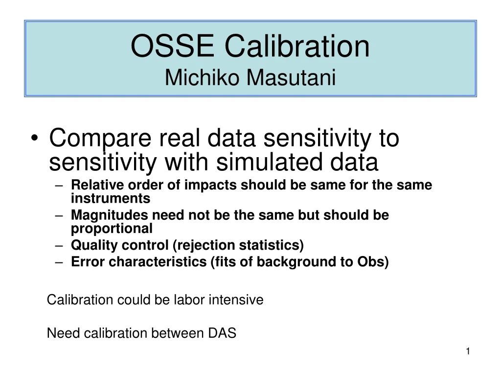
OSSE CalibrationMichiko Masutani • Compare real data sensitivity to sensitivity with simulated data • Relative order of impacts should be same for the same instruments • Magnitudes need not be the same but should be proportional • Quality control (rejection statistics) • Error characteristics (fits of background to Obs) Calibration could be labor intensive Need calibration between DAS
NH SH Calibration of Simulated Data Impacts Vs RealProblem of constant SST in T213 NR 500 hPa Height Anomaly Correlation 72 hour forecasts
Difference between analysis with real and constant SST. Time- Longitude section of 500hPa height. Averaged between 20S and 80S. Feb. 13 Real With TOVS Simulated with TOVS Mar. 7 Feb. 13 Simulated w/o TOVS Real w/o TOVS Mar. 7
SST and Impact of TOVS Anomalous warm localized SST in SH Pacific in REAL SST. In simulation experiment constant SST is used. Four analyses are performed with real SST, constant SST, with and w/o TOVS. With TOVS data the difference is small in mid troposphere but without TOVS data, large differences appear and propagate. Four experiments are repeated for simulated data. This atmospheric response to SST is reproduced by simulated experiments. Impact of TOVS is much stronger in real atmosphere. With variable SST TOVS radiance become much more important.
Observational Error FormulationSurface & Upper Air Simulated with Systematic representation error Z • With random error: • Data rejection rate too small (top) • Fit of obs too small (bottom) time
Effect of Observational Error on DWL Impact Total • Percent improvement over Control Forecast (without DWL) • Open circles: RAOBs simulated with systematic representation error • Closed circles: RAOBs simulated with random error • Orange: Best DWL • Purple: Non- Scan DWL Wave 10-20 Forecast length
Observational Error FormulationSurface & Upper Air Observation simulated at the Nature Run Surface Nature Run NCEP Model Observation simulated at the Real Surface Real
Impact of Different Surface and observational Errors (obs-anl) error [with real sfc] Random error [with real sfc] Perfect [with real sfc] Random error [with NR sfc] Real data
Data and model resolution OSSEs with Uniform Data More data or a better model? Fibonacci Grid used in the uniform data coverage OSSE • 40 levels equally-spaced data • 100km, 500km, 200km are tested Skill is presented as Anomaly Correlation % The differences from selected CTL are presented - Yucheng Song Time averaged from Feb13-Feb28 12-hour sampling 200mb U and 200mb T are presented
U 200 hPa 500km T62L64 anal and fcst 500km T62L64 anal T62L28 fcst T170Conv+TOVS 1000km T62L28 anal T62L28 fcst T62 Conv+TOVS CTL T62 Conv only 500Km T170L42 anal and fcst 200Km T170L42 anal T62L28 fcst 500Km T170L42 anal T62L28 fcst 1000km T170L42 anal T62L28 fcst CTL T170Conv+TOVS T62 Conv+TOVS NH averaged forecast skill with current observins system is close to 1000km Uniform observation
U 200 hPa Benefit from increasing the number of levels 5 500km Raob T62L64 anal T62L64 fcst L64 anl&fcst 500km Raob T62L64 anal T62L28 fcst 500km RaobT62L28 anal & fcst L64 anl L28 fcst 1000km RaobT170L42 analT62L28 fcst CTL 1000km RaobT62L28 anal & fcst T 200 hPa L64 anl&fcst 500km obs T170 L42 model High density observation give better analysis but it could cause poor forecast High density observations give a better analysis but could cause a poor forecast Increasing the vertical resolution was important for high density observations L64 anl L28 fcst
Basic Calibration Proposal • CTL: All conventional data • Suggested data types to be included • adpupa, adpsfc, satwind, aircar, aircft, sfcshp • MODIS wind • EXP1: No RAOB Wind • EXP2: NO RAOB Temp • EXP3:1000km 31 level uniform OBS Use CTL-EXP3 for inter DAS comparison