Download
1 / 97
1.17k likes | 1.5k Views
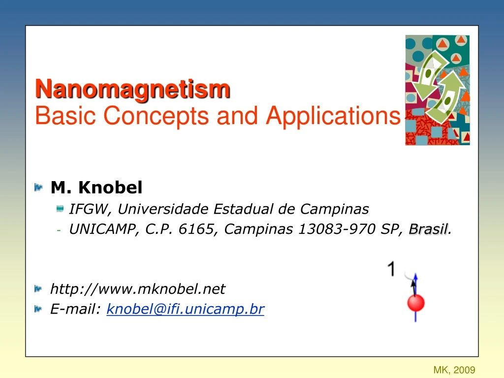
Nanomagnetism Basic Concepts and Applications. M. Knobel IFGW, Universidade Estadual de Campinas UNICAMP, C.P. 6165, Campinas 13083-970 SP, Brasil . http://www.mknobel.net E-mail: knobel@ifi.unicamp.br. Outline. Introduction M otivation Granular systems Superparamagnetism

E N D
NanomagnetismBasic Concepts and Applications • M. Knobel • IFGW, Universidade Estadual de Campinas • UNICAMP, C.P. 6165, Campinas 13083-970 SP, Brasil. • http://www.mknobel.net • E-mail: knobel@ifi.unicamp.br
Outline • Introduction • Motivation • Granular systems • Superparamagnetism • Basic concepts • Measurements • Applications • Magnetic recording • MR • Magnetic Fluids • Medicine • Etc… Co0.27(SiO2)0.73 LME-LNLS
Introduction “Extended” Ferromagnet (D) • Ferromagnetic Particle (D=D0) • Role of particle size • Both aspects (ferro+para) if D sufficiently small: Ferromagnetic Properties: • Role of anisotropies (shape, crystalline, stress, ..) • Role of magnetostatic energy Paramagnetic Properties: • Disordered state • Reversible effects Tc T Ferromagnet • Ordered State • Hysteresis (irrev. proc.) • Anisotropy (easy directions) Paramagnet • Disordered state • Reversible proc. • Isotropy
easy direction Influence of Grain Size • All particle moments rigidly aligned • Coherent rotations of = A naïve view classical vector Decreasing D • Fine particles with domains. • Single domain fine particles (Blocked state) • Superparamagnetic Regime “ free rotation” of the moment by effect of thermal disorder
Magnetic Moment Case of Co atoms M=N x 1.64m B N is of the order of 1000 atoms. The grain is a big magnetic moment which produces a magnetic field (magnetic field of a big dipole) One magnetic grain (spherical nanomagnet) is a ferromagnetic monodomain of N atoms. 3nm P. Vargas
Magnetostatic Energy and Domain Structure • Uniaxial Anisotropy: • Formation of domains reduces the magnetostatic energy. • Each new domain wall adds further energy. Where is the domain wall energy per unit area of wall, L is the thickness of the crystal and D is the thickness of the slab-like domains. For Cobalt, =7.6 ergs/cm2, L=1 cm D=1.510-3cm, i.e., 700 domains in a 1 cm cube crystal
Magnetostatic Energy and Domain Structure • Ratio of the total energy, before and after the division into domains (for Cobalt): • Further reduction in energy results from the formation of curved walls and spike domains, where unlike poles mix more intimately. • Cubic Crystals: Formation of closure domains Cullity, Introduction to Magnetic Materials, p.302 Cullity, Introduction to Magnetic Materials, p.303
Single-Domain Particles • as L becomes smaller the reduction in energy becomes smaller: at very small L the crystal prefers to remain in the single-domain state. • Moderate crystal anisotropy (Fe and Ni): Lc=100-500 A, equal to the domain wall thickness. • High crystal anisotropy (Co): Ka is large, then is large, and the wall thickness is small. Lc=500-1000 A, several times the value of . • If MS is small, a SDP can become larger without much increase of magnetostatic energy (barium ferrite vs Co). • Shape:a rod-shaped particle can have a critical diameter several times that of a sphere. Valid for high crystal anisotropy
Single Domain vs. Multi-domain • The critical size for multi-domain single domain transition: • Balance of Magnetostatic + Anisotropy + Domain wall Energy • This critical size strongly depends on the strength of anisotropy torque: • uniaxial crystalline (Ku) • cubic crystalline (K1) • Ka • shape (uniaxial); • stress (uniaxial); a b
Distinctive Aspects a) Monodomain, Blocked State • Hysteresis loop • Hc 0 • MR 0 b) Monodomain, Superparamagnetic • No hysteresis (reversibility) Energy density volume OR (And) Uniaxial Crystalline Anisotropy Spherical Shape Shape Anisotropy Elongated Particle
KAV 0 Thermally Activated Jump Thermally Activated Jump (Classical Behaviour!!) Jump frequency: Relaxation time: theoretical predictions: 0=10-9 10-10 (see later)
Demagnetization rate of an assembly of uniaxial particles f0 : frequency factor ( 109 sec-1) : relaxation time Turn-off external field at t = 0 with Mi : time for Mr to decrease to 1/e of its initial value For Co (K = 4.5106 ergs/cm3) at room temp. (T = 300 K) (V = 1.6 10-19 cm3) D = 68 Å An assembly of such particles would reach thermal equilibrium state (Mr = 0) almost instantaneously. No hysteresis
Magnetization Relaxation • Two Regimes: • Define a critical volume at constant T (e.g., RTT0) by requiring= tm : Standard Magnetic Measurements:tm 100 s Mössbauer: tm 10-8 s tm < tm > tm time Superparamagnetic Measuring time (time needed to do a measurement) Blocked For tm 100 s: 10-10
Magnetization Relaxation Define a Blocking Temperature for a given V=V0 by requiring = tm: Cullity, Introduction to Magnetic Materials, p. 415 For tm 100 s
Equilibrium Properties (static) A) Magnetization M(H, T) • Classical treatment Langevin Function It is a crude approximation: i) Moments distributed p() ii) Interactions neglected Often: ... but interactions are still neglected.
Testing Superparamagnetism • Plot m =M/MS vs. H/T ,if curves superimpose, OK!! Deviations to be ascribed to blocked particles and/or interactions Cullity, Introduction to Magnetic Materials, p. 412
Langevin Function But n is the maximum possible moment which the material can have, corresponding to the perfect alignment of the moments to the field (saturation magnetization M0). Langevin Function Series expansion: Curie Law: For small a, L(a)=a/3: M0 being the saturation magnetization of the alloy, and MS the saturation magnetization of the element
Langevin Function C.L. Chien, Annu. Rev. Mater. Sci. 1995. 25:129-60 Influence of the particle diameter
Curie Law • Non-interacting granules, T>TB: • For interacting granules [Chantrell and Wohlfarth, J. Magn. Magn. Mater. 40, 1, 1983]: • Because of the temperature dependence of MS(T), 1/ is not linear with T. • T0 can be obtained in the plot 1/ vs T, when 1/ reduces to zero. • Once T0 is obtained, one can deduce MS(T), normally a Bloch´s law: Curie-Weiss type
Equilibrium Properties B) ZFC and FC curves sample cooled in zero field from T1 (where all particles are S.P.) to Tmin (at constant rate) small measuring field applied at Tmin sample heated from Tmin up to high T and M measured (ZFC magnetization) sample cooled under an external magnetic field from T1 to Tmin at constant rate sample heated from Tmin to high T and M measured (FC magnetization) ZFC FC
Equilibrium Properties ZFC and FC curves Above Tirr, is so short that thermal equilibrium is always attained before completing a single measurement (SuperParamagnetic state) TM 1 Isothermal Relaxation under field Isochronal Relaxation under field Tirr 1 2 2 Tmin Tirr TMAX TB Blocking Temperature Curves are degenerated above TirrTMAX
Zero Field Cooling Magnetization (ZFC) (3) ZFC H (4) (2) H H = 0 (1) J.C.Denardin, A.L. Brandl, M. Knobel et al, Phys. Rev. B 65, 64422 (2002)
Field Cooling Magnetization (FC) H FC H (5) ZFC J.C.Denardin, A.L. Brandl, M. Knobel et al, Phys. Rev. B 65, 64422 (2002)
Simulated ZFC/FC and TRM curves TB=30 K =0.4 In collaboration with Dr. Pierre Panissod
Equilibrium Properties Attention: Irreversibility and cusp-like features could also indicate spin-glass transitions. Apparent irreversibilities appear when TB is not attained (point f). C.L. Chien, Annu. Rev. Mater. Sci. 1995. 25:129-60
Experiment: M(H,T) particle moment
Experiment: M(H,T) tm > superparamagnetic regime tm < blocked regime FC ZFC TB Roberto Zysler
Off-Equilibrium Properties (Relaxation) A) Relaxation of Remanence • At a given T and H one has: • When H=0, MSP=0 and • TRM (ThermoRemanent Magnetization) • sample cooled from T1 (S.P. regime) down to measuring T (Tmeas<TB) under field. • Field removed at T=Tmeas • MR relaxing.
Thermoremanent Magnetization (TRM) = 0.5 (uniaxial anisotropy) • sample is cooled (2 K); • with a high applied field (40 KOe); • the field is set to zero and after • 100 s the remanent magnetization is measured; • this procedure is reapeated for each T. H = 0 J.C.Denardin, A.L. Brandl, M. Knobel et al, Phys. Rev. B 65, 64422 (2002)
Off-Equilibrium Properties (Relaxation) Relaxation of Remanence • Single volume Distributed volumes but often logarithmic laws are found (in certain time domains): Follows Arrhenius law Evidence of a broad distribution of volumes or of correlated relaxation processes.
Off-Equilibrium Properties (Relaxation) B) A.C. Susceptibility Application of a very small AC field allows the initial susceptibility ito be measured (using the expression of in the absence of field. Possibility to explore a very large time window, changing the frequency of the AC field. Susceptibility of an assembly of non-interacting single domain particles: • If <<1, ´= 0 (susceptibility in the S.P. regime, reversing many times during the measuring time tm). • If >>1, ´= 1, susceptibility in the blocked regime, where the moments don´t reverse during tm. Real part:
Off-Equilibrium Properties (Relaxation) A.C. Susceptibility • ´ is expected to show a maximum at a temperature TM close to <TB>. • For uniaxial anisotropy: according to the Arrhenius law. A=1.8-2.0 depending on the used distribution function Frequency independent at high temperatures TM shifts towards higher Temperatures and decreases, for increasing frequencies
Classical Dynamics of Moments (S.P.) Under magnetic field: (precession around field axis) • All atomic moments within a single particle are precessing coherently (sort of Ferromagnetic precession mode, like in ferromagnetic resonance) • Giromagnetic ratio • Frequency of precession for a single : for H=104 Oe L 1011 s-1 Precession time: Larmor frequency
Classical Dynamics of Moments (S.P.) • Disturbances to Coherent Rotation: • Moment - Lattice Interactions 1: moment-lattice relaxation time (practically coincident with the moment reversal time calculated by Brown and Néel 1 10-10 exp[KaV/kBT], and thus depends on the particle´s volume) • Moment - Moment Interactions 2: moment-moment relaxation time (local field generated by interactions disturbs the phase angle) Dipolar interactions: Hi 1000 Oe, 210-10 s • For “large” particles (d>6 nm): 1>2 • For “small” particles (d<2 nm): 1<2
Relaxation Time • Néel´s view (1949) • Assumptions: • EA>> kBT (spins nearly aligned along easy direction) • s 0 The particle is strained along z (not shown) The energy barrier always increases due to magnetoelastic effects The particle is strained along z (not shown)
Relaxation Time • Brown´s view (1963) • Micromagnetic approach: continuous vector field M • A stochastic Gilbert equation for M: • If = KaV / kBT >> 1 : Giromagnetic constant Anisotropy field Random “field” Damping (Ferromagnetic Particles, Uniaxial anisotropy)
Size Distribution It is difficult make samples with monodisperse grain sizes Granular systems are well described by a log-normal distribution function:
Distribution Function Log-normal distribution function:
Nanocrystalline Materials • Grain size distribution • Distribution of magnetization easy-axes • Magnetic interactions • Surface effects • Matrix effects
Nanocrystalline materials • Metal-insulator transition • Giant (tunneling) magnetoresistance • Giant Hall effect • Superparamagnetism • Magnetic interactions • Metallic conduction • “bulk” magnetism • Anisotropic magnetoresistance Cox[SiO2]1-x x = 0.72 x = 0.28 x = 0.62
Magnetization Rotation How does the magnetization really rotate? Modes of Superparamagnetic Relaxation (for an elongated ellypsoid): • Coherent Rotation (rotation in unison) • Incoherent Rotation • Fanning • Curling • Buckling a) Coeherent Rotation The exchange energy remains a constant There is a temporary increase in Magnetostatic Energy This is the typical relaxation mode for ultrafine particles (<15 nm for Fe)
Magnetization Rotation b) Incoherent Rotation • Curling-mode reversal The spins twist in a non-coherent manner around the easy axis. The exchange energy is no more constant. Na extra magnetostatic energy is present. However: Em(curling)<Em(unison) The curling mode reversal occurs in larger particles (1020 nm) Cullity, Introduction to Magnetic Materials, p. 394.
Magnetization Rotation b) Incoherent Rotation • Fanning-mode reversal • Chain of spheres model (Jacobs and Bean) Intrinsic Coercivity (diameter a and field applied along the chain): Cullity, Introduction to Magnetic Materials, p. 390, 392.
Magnetization Rotation Intrinsic Coercivity (diameter a and field applied along the chain): A) Fanning : B) Coherent Rotation: Cullity, Introduction to Magnetic Materials, p. 390, 392. 3 times Larger
Magnetization Rotation • Size dependence: comparison among the different modes Cullity, Introduction to Magnetic Materials, p. 396, 397.
very small particles surface influence Is it a perfect magnetic order? Roberto Zisler
FIG. 2. Color online a Symbols: ZFC-FC magnetization curves measured under applied field of H=20 Oe. Solid lines: simulated ZFC-FC curves using the NP size distributions observe by TEM. b Experimental ac susceptibility vs temperature measured using an oscillating field with magnitude of 7 Oe. FIG. 1. TEM image of the Ni NPs used in this work. Inset: HRTEM image showing that the NPs have a complex internal structure. FIG. 3. Color online ZFC and FC magnetization curves of the Ni NPs for different values of dc magnetic fields. W. C. Nunes, E. De Biasi, C. T. Meneses, M. Knobel, H. Winnischofer, T. C. R. Rocha, D. Zanchet, Appl. Phys. Lett. 92, 183113 (2008).
Coercivity of Fine Particles Striking dependence on the particle size Fig. 11.1 The coercivities vary over three orders of magnitude and the particle sizes over five. Smallest size: 10 unit cells, Largest size: 0.1 mm The mechanism of magnetization differs from one part of the size range to another.