Download
1 / 54
540 likes | 549 Views
Math.375 Interpolation. Vageli Coutsias, Fall `05. function plot_temp() [L,K,T] = av_temp plot(L,T(:,1),'g',L,T(:,2),'r',L,T(:,3),'b',L,T(:,4),'k') title(' The temperature as a function of latitude ') xlabel(' Latitude (in degrees) ') ylabel(' Temperature ')

E N D
Math.375 Interpolation Vageli Coutsias, Fall `05
function plot_temp() [L,K,T] = av_temp plot(L,T(:,1),'g',L,T(:,2),'r',L,T(:,3),'b',L,T(:,4),'k') title(' The temperature as a function of latitude ') xlabel(' Latitude (in degrees) ') ylabel(' Temperature ') legend('K=.67','K=1.5','K=2.0','K=3.0') function [L,K,T] = av_temp % Q&S Table 3.1 L = 65:-10:-55; K = [.67, 1.5,2.0,3.0]; % T is 13x4 T = [-3.10, 3.52, 6.05, 9.30;... -3.22, 3.62, 6.02, 9.30;... -3.30, 3.65, 5.92, 9.17;... -3.32, 3.52, 5.70, 8.82;... -3.17, 3.47, 5.30, 8.10;... -3.07, 3.25, 5.02, 7.52;... -3.02, 3.15, 4.95, 7.30;... -3.02, 3.15, 4.97, 7.35;... -3.12, 3.20, 5.07, 7.62;... -3.20, 3.27, 5.35, 8.22;... -3.35, 3.52, 5.62, 8.80;... -3.37, 3.70, 5.95, 9.25;... -3.25, 3.70, 6.10, 9.50];
Topics • Polynomial Interpolation in 1d: Lagrange & Chebyshev • POLYFIT & POLYVAL • 2D: Matrices and Color Images • Trigonometric Interpolation • Sound
function runge1() close all a = -1; b = 1; m = 17; %Equally Spaced, m=17 x = linspace(a,b,m); y = rung(x, 16); x0 = linspace(-1,1,100); y0 = rung(x0,16); [P,S] = polyfit(x,y,17); pVal = polyval(P,x0); plot(x,y,'ro',x0,pVal,'b',x0,y0,'r--') axis([-1,1,-2,2]) function y = rung(x,a) y = 1./(1+a*x.^2);
[P,S] = polyfit(x,y,17); pVal = polyval(P,x0);
% least squares fit: degre 8 fit based on 17 pts. [P,S] = polyfit(x,y,8); pVal = polyval(P,x0);
for i = 1:m+1 % Chebyshev Nodes x(i,1) = .5*(b+a) +.5*(b-a)*cos(pi*(i-1)/m) ; end y =1./(1+16*x.^2); [P,S] = polyfit(x,y,17); pVal = polyval(P,x0);
Machine assignment 2.7 (a) Write a subroutine that produces the value of the interp. polynomial at any real t, where is a given integer, are n+1 distinct nodes, and f is any function available in the form of a function subroutine. Use Newton’s interpolation formula and generate the divided differences (from the bottom up) “in place” in single array of dim n+1 that originally contains the function values. (b) Run your routine on the function using and n=2:2:8 (Runge) Plot the polynomials against the exact function.
function c = InterpNRecur(x,y) n = length(x); c = zeros(n,1); c(1) = y(1); if n > 1 c(2:n) =InterpNRecur(x(2:n), ((y(2:n)-y(1))./(x(2:n)-x(1))); end
function c = InterpN(x,y) n = length(x); for k = 1:n-1 y(k+1:n) = (y(k+1:n)-y(k))/(x(k+1:n)-x(k)); end c = y;
function pVal = HornerN(c,x,z) n = length(c); pVal = c(n)*ones(size(z)); for k=n-1:-1:1 pVal = (z-x(k)).*pVal + c(k); end
% Ma505; Gautschi M.2.7 for m=1:4 n=2*m; x = linspace(-5,5,n+1); y = 1./(1+x.^2); x0 = linspace(-5,5,1000); y0 = 1./(1+x0.^2); a = InterpNRecur(x,y); pVal = HornerN(a,x,x0); subplot(2,2,m) plot(x0,y0,x0,pVal,'--',x,y,'*') axis([-5 5 -1 1]) end
Lagrangian Polynomial Interpolating Polynomial is a UNIQUE polynomial of degree n that agrees with f(x) at the n+1 nodes
Problem 2.24 Prepare plots of the Lebesgue function for interpolation, for with the nodes given by: Compute on a grid obtained by dividing each interval into 20 equal subintervals. Plot in case (a) and in case (b).
The Lebesgue function and constant for a grid are defined as: with the Lagrange polynomial: Below we give a matlab script that computes the Lebesgue functions (and constants) for the given grids.
% Math 505; Gautchi 2.24: Lebesgue functions fprintf(' n equispaced Chebyshev \n') for ii=0:2 n=5*2^ii; xa(1:n+1,1)=0; xb(1:n+1,1)=0; for i= 1:n+1 xa(i,1) = -1+2*(i-1)/n; xb(n+2-i,1) = cos(pi*(2*(i-1)+1)/(2*n+2)); end for i=1:n for j=1:20 ga(20*(i-1)+j,1)=((21-j)*xa(i)+(j-1)*xa(i+1))/20; gb(20*(i-1)+j,1)=((21-j)*xb(i)+(j-1)*xb(i+1))/20; end end ga(20*n+1,1)=xa(n+1); gb(20*n+1,1)=xb(n+1); for k = 1:20*n+1 %compute Lebesgue functions na(:,k)=ga(k)-xa(:); nb(:,k)=gb(k)-xb(:); %numerators end for i = 1:n+1 % denominators for j=1:n+1 da(i,j) = xa(i)-xa(j); db(i,j) = xb(i)-xb(j); end end
for k = 1:20*n+1 for i = 1:n+1 la(i,k) = 1; lb(i,k) = 1; for j=1:n+1 if j~=i la(i,k)=la(i,k)*na(j,k)/da(i,j); lb(i,k)=lb(i,k)*nb(j,k)/db(i,j); end end end lama(k)=1; lamb(k)=1; for i=1:n+1 lama(k)=lama(k)+abs(la(i,k)); lamb(k)=lamb(k)+abs(lb(i,k)); end end figure subplot(2,1,1); plot(ga,log(lama)) subplot(2,1,2); plot(gb,lamb) lamax =lama(1); lambx =lamb(1); % compute Lebesgue constants for k = 2:20*n+1 if lama(k) > lamax; lamax= lama(k); end if lamb(k) > lambx; lambx= lamb(k); end end fprintf('%9i %22.14f %22.14f \n',n,lamax,lambx); clear end
a b n=5 n=10 Lebesgue constants n equispaced Chebyshev 5 4.10496 2.68356 10 30.8907 3.06859 20 10987.5 3.47908 The plots give the Lebesgue fncs (log of same for grid (a)). a b n=20
Fourier series
Band Limited Functions Complex Form
f t
The Fast Fourier transform • fft: compute Fourier coefficients from sampled function values • ifft: reconstruct sampled values from (complex) coefficients • interpft: construct trigonometric interpolant
FFT Discrete Fourier transform. FFT(X) is the discrete Fourier transform (DFT) of vector X. For length N input vector x, the DFT is a length N vector X, with elements N X(k) = sum x(n)*exp(-j*2*pi*(k-1)*(n-1)/N), 1 <= k <= N. n=1 The inverse DFT (computed by IFFT) is given by N x(n) = (1/N) sum X(k)*exp( j*2*pi*(k-1)*(n-1)/N), 1 <= n <= N. k=1 See also IFFT, FFT2, IFFT2, FFTSHIFT.
INTERPFT 1-D interpolation using FFT method. Y = INTERPFT(X,N) returns a vector Y of length N obtained by interpolation in the Fourier transform of X. Assume x(t) is a periodic function of t with period p, sampled at equally spaced points, X(i) = x(T(i)) where T(i) = (i-1)*p/M, i = 1:M, M = length(X). Then y(t) is another periodic function with the same period and Y(j) = y(T(j)) where T(j) = (j-1)*p/N, j = 1:N, N = length(Y). If N is an integer multiple of M, then Y(1:N/M:N) = X.
function F =CSInterp(f) n = length(f); m = n/2; tau = (pi/m)*(0:n-1)'; P = []; for j = 0:m, P = [P cos(j*tau)]; end for j = 1:m-1, P = [P sin(j*tau)]; end y = P\f; F = struct('a',y(1:m+1),'b',y(m+2:n));
THE FOURIER COEFFICIENTS F.a=[y(1),…,y(m+1)] F F.b=[y(m+2),…,y(2m)] A CELL array: it’s elements are STRUCTURES (here arrays) F = struct('a',y(1:m+1),'b',y(m+2:n));
function Fvals = CSeval(F,T,tvals) Fvals = zeros(length(tvals),1); tau = (2*pi/T)*tvals; for j = 0:length(F.a)-1 Fvals = Fvals + F.a(j+1)*cos(j*tau); end for j = 1:length(F.b) Fvals = Fvals + F.b(j )*sin(j*tau); end
% Script File: Pallas A = linspace(0,360,13)'; D=[ 408 89 -66 10 338 807 1238 1511 1583 1462 1183 804 408]'; Avals = linspace(0,360,200)'; F = CSInterp(D(1:12)); Fvals = CSeval(F,360,Avals); plot(Avals,Fvals,A,D,'o') axis([-10 370 -200 1700]) set(gca,'xTick',linspace(0,360,13)) xlabel('Ascension (Degrees)') ylabel('Declination (minutes)')
The Gibbs Phenomenon ….
% Script File: square % Trigonometric interpolant of a square wave. M=300 A = linspace(0,360,2*M+1)'; D(2:M)=0;D(M+2:2*M)=1; D(1)=.5;D(M+1)=.5;D(2*M+1)=.5; D=D'; Avals = linspace(0,360,1000)'; F = CSInterp(D(1:2*M)); Fvals = CSeval(F,360,Avals); plot(Avals,Fvals)
…. can be seen at all discontinuities
% Script File: sawtooth_wave. clear M=512 A = linspace(0,360,2*M+1)'; D(2:M)=(2:M)/M;D(M+2:2*M)=-1+(2:M)/M; D(1)=0;D(M+1)=0;D(2*M+1)=0; D=D'; Avals = linspace(0,360,1024)'; F = CSInterp(D(1:2*M)); Fvals = CSeval(F,360,Avals); plot(Avals,Fvals)
The overshoot is present at any resolution…
…although the interpolant is correct at the nodes as dx->0
Compare with equispaced polynomial interpolation
Input-output structures • x=input(‘string’) • title=input(‘Title for plot:’,’string’) • [x,y]=ginput(n) • disp(‘a 3x3 magic square’) • disp(magic(3)) • fprintf(‘%5.2f \n%5.2f\n’,pi^2, exp(1))
Writing to and reading from a file fid = fopen('output','w') a=linspace(1,100,100); fprintf(fid,'%g degC = %g degF\n',a,32+1.8*a); fid=fopen('output','r') x=fscanf(fid,'%g degC = %g degF'); x=reshape(x,(length(x)/2),2)
---------------------------------------- I. A=[1 2 3;4 5 6;7 8 9]; y=x'; %transpose x=zeros(1,n); length(x); x=linspace(a,b,n); a=x(5:-1:2); %SineTable (Help SineTable) disp(sprintf('%2.0f %3.0f ',k, a(k))); ----------------------------------------