Download

1 / 39
390 likes | 667 Views
Markov Models (Basics). Markov Models. Markov Decision Process (MDP). No observation uncertainty, with decision. With observation uncertainty, no decision. Partially Observable Markov Decision Process (POMDP). Markov Chain (MC). Hidden Markov Model (HMM).

E N D
Markov Models Markov Decision Process (MDP) No observation uncertainty, with decision With observation uncertainty, no decision Partially Observable Markov Decision Process (POMDP) Markov Chain (MC) Hidden Markov Model (HMM) With both observation uncertainty and decision 2
Markov Chain • Definition • For a time series, , • Components • System states • Example: {cold, warm, hot} • Transition probability • Example: 3
Hidden Markov Model (HMM) • States: • Observations: • The system state is the underlying rule of the real world, which is not visible and can only be estimated using observations (associated with uncertainties). • Components: • State: • Observation: • State Transition Probability: • Observation Probability: 4
An Example of HMM • Estimate the climate using the tree ring • States: {H(hot), C(Cold)}. • Observation (size of tree ring): {L(large),M(medium), S(small)} • State Transition: • Observation: 5
Solving HMM Problems • State Transition: • Observation: • The initial distribution of states is {P(H)=0.6,P(C)=0.4}. Suppose that our observation is {S,M,S,L} in four years, what are the corresponding climate? • P(HHCC)=P(H)*P(S|H)*P(H|H)*P(M|H)*P(C|H)*P(S|C)*P(C|C)*P(L|C) • = 0.6*0.1*0.7*0.4*0.3*0.7*0.6*0.1=0.000212 • We compute the probability corresponding to each possible sequence such as P(HHHH), P(HHCH), P(HCHC), … 6
Solving HMM by Enumeration • Among all the state sequences, CCCH has the largest probability. Thus it should be chosen as the estimated state sequence. • This solving process needs to compute the probability of sequences if is the length of sequence and is the number of system states. The complexity is exponential. Stamp, Mark. "A revealing introduction to hidden Markov models." 7
Solving HMM by Dynamic Programming • The first year observation is S • P(H)=0.6*0.1=0.06, P(C)=0.4*0.7=0.28 • The second year observation is M • P(HH)=0.06*0.7*0.4=0.0168 • P(HC)=0.06*0.3*0.2=0.0036 • P(CH)=0.28*0.4*0.4=0.0448 • P(CC)=0.28*0.6*0.2=0.0336 Pruned since those two sequences cannot appear in the optimal sequence Each step, we only keep two sequences with the largest probabilities among those ending with H and C. 8
Markov Decision Process (MDP) • Given the current state and state transition probability matrix, MDP is to determine the best decision which leads to the maximum expected reward • There is no observation or observation uncertainties 9
Partially Observable Markov Decision Process (POMDP) • POMDP • Given the current observation (with uncertainties) and state transition probability matrix, POMDP is to determine the best decision which leads to the maximum expected reward • Model the past, model the present and predict the future (probabilistic long term reward) • Three layer architecture • Observation, State, Action • POMDP models the interactions among them 10
A Simple Example of POMDP , : No hacking, , : Smart meter 1 is hacked, , : Smart meter 2 is hacked. , : Both smart meters are hacked. : No or negligible cyberattack, : Check and fix the hacked smart meters 11
Output of POMDP: Policy Transfer Graph Policy: a set of actions where there is a corresponding action for each possible state 12
Modeling The Past: Probabilistic State Transition Diagram 0.5|,1| • Learn from historical observation data • Calibrate mapping from observation to state • Apply conditional probability (Bayesian rule) 0|,1| 0|,1| 0|,1| 0.1|, 0| 0.2|, 0| 0.2|, 0| 0|, 0| 0|, 0| 0.5|, 0| 0.5|, 0| 1|, 0| 0|, 0| 0.1|, 0| 0.5|, 0| 0.5|, 0| 13
Modeling The Present • Belief State: we know the current state in a probabilistic sense • The probabilistic distribution over states • [0.7, 0.15, 0.05, 0.1] is a belief state, meaning that 70% chance in s0, 15% in s1, 5% in s2 and 10% in s3. 14
Predict The Future Account for the Future 15
Find a Series of Actions w/ Maximum Reward in Future Associate a reward to each action and weight it differently at different time slot. Find a series of actions leading to the maximum reward for the future k time slots. After an action, the new belief state is 1 for 2pm Discount Factor: 0.5 0.5 for 3pm < > 0.25 for 4pm < 0.125 for 5pm > < < < 16
The POMDP Formulation • A POMDP problem is formulated as • : The system state space. • : The action space. • : The observation of the system state. • : The state transition function, defined as the probability that the system transits from state to when action is taken. • : The observation function, defined as the probability that the observation is when the state and action are and respectively. • : The reward function, defined as the reward achieved by the decision maker, taking action at state which transits to . 17
Belief-State MDP • Using the belief state, the POMDP problem is reduced to • : The space of belief state • Given a new observation, the belief state is updated as • : The intermediate reward for taking action in the belief state • (1) • : The transition function between the belief states • (2) • Filtering (monitoring) to track belief states • Stochastic and statistical filtering, e.g., Kalman filter (optimal when belief states are Gaussian, transition function is linear, and MDP is still discrete time), Extended Kalmanfilter or particle filter 18
Probabilistic State Transition Computation • When • (3) • (4) • Compute directly? • The action does not change the state, so we can obtain the state transition from the observation transition. • (5) • (6) • is approximated by 19
Reward for Future • POMDP aims to maximize the expected long term reward (Bellman’s Optimality), where is a discount factor to reduce the importance of the future events, and is the reward achieved in step . • Reward for each action • (7) • (8) System loss when there is an undetected cyberattack Labor cost due to detection 20
Obtain the training data Obtain the Observation Estimate the state transition probability for action using according to Eqn. (5) and Eqn. (6) Map the observation to belief state Reset state transition probability and observation probability for from Eqn. (3) and Eqn. (4) respectively. Compute the belief state transition according to Eqn. (2) Obtain the reward functions according to Eqn. (7) and Eqn. (8) respectively. Compute the intermediate reward function according to Eqn. (1) ? No IYes Apply single event defense technique on each smart meter to check the hacked smart meters and fix them. Solve the optimization problem P to get the optimal action 21
pomdp.m 23
recursive.m 24
Input and Output of pomdp.m • Input • gamma is the discount factor, O is the observation function, R is the reward function and T is the state transition. • A is the set of the available actions. ob is the previous belief state, oc is the current observation (given), and oais the previous action. • Output • table is the expected reward of each action and b is the updated belief state. 25
Denotations in MATLAB • T(i,j,a) • O(i,j,a) • R(i,j,a) 26
Recursively Compute Expected Reward • gamma is the discount factor 28
Input and Output of recursive.m • a is the action in the last step • gamma is the discount factor and r is the cumulative discount factor • Other inputs are defined the same as before • reward is the expected reward of the subtree 29
Recursively Compute Expected Reward Associate a reward to each action and weight it differently at different time slot. Find a series of actions leading to the maximum reward for the future k time slots. For each action, belief state is predicted by 1 for 2pm Discount Factor: 0.5 0.5 for 3pm < > 0.25 for 4pm < 0.125 for 5pm > < < < 30
Belief State Prediction • bx=b*T(:,:,a) : • for i=1:N • bx(i)=0; • for j=1:N • bx(i)=bx(i)+b(i)*T(j,i,a); • end • end 32
Recursive Call • r*recursive(R,T,A,bx,i,gamma,r*gamma): • Compute the expected rewards of subsequent subtrees • b*sum(R(:,:,a).*T(:,:,a),2): • Compute the instant reward, which is the expectation of the rewards over all the possible next states 33
Detection in Smart Home Systems I Initialization Observation, Obtained from Smart Home Simulator Call POMDP for Smart Home Cyberattack Detection 34
Bottleneck of POMDP Solving • The time complexity of the POMDP formulation is exponential to the number of states. • There can even be exponential number of states and thus the size of the state transition probability matrix. • Speedup techniques are highly neccessary.
Speedup is All About Mapping • Find a series of actions w/ maximum reward in the belief state space • The corresponding maximum reward is called value function V* • Value function is piece-wise linear and convex. • Cast a discrete POMDP with uncertainty into an MDP defined on belief states, which is continuous and potentially easier to approximate. All about mapping between b and V*(b) Value function V* Belief state space 36
Idea #1: ADP for Function and Value Approximation • Function approximation: round V*(b) • Compute V*(b’) on a set of selected grid points b’ in the belief state space • Perform regression to approximate V*(b) function for all other b • Polynomial, RBF, Fourier, EMD • RL or NN • Value approximation: round b • Get a set of samples B, and precompute V*(B) • Given a request b, computes b' as the nearest neighbor from samples and return V*(b') Value function V* Belief state space 37
Idea #2: ADP for Policy Approximation < Reward is too small < Reward is too small < 38