Download
1 / 43
430 likes | 577 Views
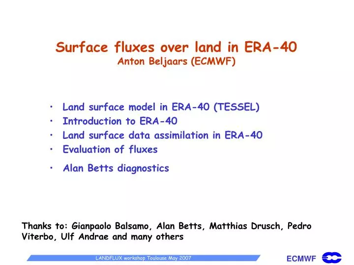
Surface fluxes over land in ERA-40 Anton Beljaars (ECMWF). Land surface model in ERA-40 (TESSEL) Introduction to ERA-40 Land surface data assimilation in ERA-40 Evaluation of fluxes Alan Betts diagnostics.

E N D
Surface fluxes over land in ERA-40Anton Beljaars(ECMWF) • Land surface model in ERA-40 (TESSEL) • Introduction to ERA-40 • Land surface data assimilation in ERA-40 • Evaluation of fluxes • Alan Betts diagnostics Thanks to: Gianpaolo Balsamo, Alan Betts, Matthias Drusch, Pedro Viterbo, Ulf Andrae and many others
Why is the land problem so difficult compared to the ocean problem? Fluxes can be written as: Lowest model level U1,V1,T1,q1 z1 0, 0, Ts, qs Surface
The land surface scheme (TESSEL) No root extraction or deep percolation in frozen soils Climatological land use data fields derived from 2’30” GLCC: Low vegetation cover High vegetation cover Low vegetation type High vegetation type High vegetation Low vegetation Interception reservoir Bare soil Exposed snow Snow under high vegetation Lowest model level Aerodynamic resistances depend on: roughness lengths and stability Snow under high vegetation has low albedo Canopy resistances depend on: radiation, air humidity, soil water (not ice) Root depth depends on vegetation type One global soil type: loam
Snow model in TESSEL (2 tiles) Single layer snow pack with prognostic equations for (Douville et al. 1995): • Snow mass (right hand side : snow fall, snow melt and snow evaporation) • Snow temperature (right hand side: radiative heating, turbulent fluxes, basal heat flux) • Snow density (right hand side: decrease to min 100 kg/m2 for fresh snow; relaxation to 300 kg/m2 in 3 days) • Snow albedo (right hand side: reset to 0.85 for fresh snow, relaxation to 0.50 with a time scale of a month for cold snow and about 4 days for melting snow) • Snow depth D from mass and density • Snow cover increases linearly with snow mass (total cover at 15 kg/m2) Snow albedo is only used for “exposed snow” tile Tile with snow under high vegetation has albedo of 0.2 (Viterbo and Betts, 1999) Lowest model level 7 cm 21 cm 72 cm 189 cm Snow under vegetation Exposed snow
Offline TESSEL evaluation with BOREAS data BOREAS evaporation: One-column integration TESSEL Old Jan 1994 Jan 1995 Jan 1996 • Used 9 different datasets for offline testing: • Cabauw • FIFE • BOREAS 1994-1996 • NOPEX 1994-1996 • Torne-Kalix (PILPS2E) • …. • The old model erroneously transform the available energy into evaporation. However, plants have limited transpiration in winter/spring, when the roots are frozen. • The TESSEL model simulates this because the stress function relies on available water (excluding ice). Van den Hurk et al, 2000
BOREAS: runoff vs observations • Deep drainage is the only mechanism for runoff in the old (ERA15) model (control). There is no mechanism for fast runoff and no peak associated to spring snowmelt. • TESSEL (ERA40) restricts vertical water transfer in frozen soils. Fast runoff due to: (a) snowmelt over frozen soils, and (b) Soil water melt. Betts et al, 2001. J. Geophys. Res., BOREAS special issue.
BOREAS snow depth • In the old (control) model, evaporation causes too early depletion of snow • TESSEL (new) model limits snow evaporation, and depletion of snow (by melting) occurs later Van den Hurk et al, 2000. ECMWF Tech. Mem. 295, 42 pp.
Stand alone simulation with old land surface scheme (control) and new scheme (TESSEL or tile) using long time series from Cabauw (10-day averages) The two model versions are rather similar for Cabauw van den Hurk et al. (2000)
ERA-40 analysis system • Global T159 (about 125 km resolution), 60 levels (top level at 10 Pa) 1957 - 2002 • 3DVAR with 6 hour cycling • FGAT (first guess compared to observation • at appropriate time; increment added at analysis time) • Model first guess is converted into equivalent of observation using a forward model e.g. RT model for satellite radiances • Atmospheric analysis variables: U,V,T,q,Ps,O3 • Cloud prognostic variables (cover, condensate) are not analyzed and are copied from 1st guess 0 6 12 18 0
ERA-40 analysis system • Model related parameters are computed during the first guess and during short range forecasts from 0 and 12 UTC e.g.: • precipitation • surface and top of the atmosphere fluxes • cloud variables • Model related parameters can have biases that are • related to model deficiencies • Post-processing of models fields every 3 hours for study of short time scale variability, e.g. diurnal cycles • Comprehensive set of vertically integrated fields for budget studies, e.g. moisture covergence • Some “physics” parameters (diffusion coefficients, mass fluxes, 3D precip) are archived for chemical transport modelling See: Uppala et al. 2005; QJRMS, 131, 2961-3012 and http://www.ecmwf.int/research/era
Observations • Conventional observations: • Radio-sondes, pilot winds, profilers • SYNOP’s • SHIP’s • Buoys • Aircraft reports • Satellite observations • TOVS/ATOVS radiances • Scatterometer winds • SSMI 1DVAR retrievals of TCWV and winds • Cloud track winds Density and quality of observations is (dependent on type) variable over the 40-year period
Soil moisture analysis • Soil moisture observations are not available on a global scale. • Soil moisture analysis at ECMWF uses first guess errors (6 or 12 hour forecast compared to SYNOP observations) of temperature and humidity to correct soil moisture. • Effectiveness of method depends on quality of model (particularly the land surface scheme). • Three methods have been developed at ECMWF: • (i) Nudging using q observations only (Viterbo and Courtier 1995) • (ii) OI using q and T. ERA uses OI (Douville et al. 2000) • Kalman filter developed in ELDAS; still to be implemented operationally (Sueffert et al. 2004) Boundary layer reservoir in dry day-time conditions Soil moisture reservoir The use of boundary layer q to infer soil moisture assumes a perfect relation between E and . The method may be very good for E (what we want in NWP), but not necessarily good for .
Time series of q at Cabauw (Netherlands) 200 m Above the surface Data assimilation systems are very powerful in representing synoptic variability of the main atmospheric variables (U,V,T and q). This applies in particularly to T2 RH2 due to land surface data assimilation 2 m Above the surface Data: Fred Bosveld, KNMI
Trends and interannual variability CRU/Hadley Centre http:///www.cru.uea.ac.uk/cru/info/warming ERA-40 See: Simmons et al. 2004; JGR, 109, D24
2m temperature analysis increments in ERA-40 July 1986-1995 2m relative humidity analysis increments in ERA-40 July 1986-1995
Surface analysis increments in ERA-40 (1986-1995) 2m Temperature (K/6-hours) Temperature (top 7-cm layer; K/6-hours)
Surface analysis increments in ERA-40 (1986-1995) Water (top 1m of soil; mm/6-hours ) 2m Relative humidity (%/6-hours ) Snow (mm of water equivalent/6-hours )
July fluxes (positive=up): Open loop -OI LE H Drusch and Viterbo, 2007
1000hPa RMS-T errors: Open loop versusOIEurope (dot), N-Amer(solid), E-Asia (dash) Drusch and Viterbo, 2007
Oklahoma meso-net (34N-36.8N/94.6W-99.9W); 72 stations with meteo and soil moisture. Drusch and Viterbo, 2007 OIOpen loopObserved Downward solar radiation Precipitation Soil moisture (top 5 cm) Soil moisture (top 100 cm)
Mackenzie basin averaged monthly evaporation (ERA40) Betts et al. 2003
Data from the Boreal Ecosystem Research and Monitoring Sites (BERMS) • Three different sites less than 100 km apart in Saskatchwan at the southern edge of the Canadian boreal forest (at about 54oN/105oW) : • Old Aspen (deciduous, open canopoy, hazel understory, 1/3 of evaporation from understory) • Old Black Spruce (boggy, moss understory) • Old Jack Pine (sandy soil) Thanks to the Fluxnet-Canada Research Network (A. Barr, T. A. Black, J. H. McCaughey)
BERMS vs ERA-40 (Daily averages: Apr, May, Jun) 2m temperature ERA-40 follows observations with RMS error of about 2 K. Daily averages processed by Alan betts
BERMS vs ERA-40 (Daily averages: Apr, May, Jun) Sensible heat flux (negative = up)
BERMS vs ERA-40 (Daily averages: Apr, May, Jun) Latent heat flux (negative = up)
BERMS vs ERA-40 (Daily averages: Apr, May, Jun) Ground heat flux
BERMS diurnal cycles (30-day averages) Rnet SSHF G SLHF
OBS ERA OBS ERA Cabauw (The Netherlands, 52N, 5E) 7-day averages 1986-1997 Sensible heat flux Latent heat flux
OBS ERA Norunda (Sweden, 60N, 17E) 7-day averages 1986-1997 Sensible heat flux Latent heat flux
Conclusions from ERA-40 • NWP analysis is very efficient in reproducing synoptic variability • Fluxes in ERA-40 are adjusted through soil moisture and temperature based on boundary layer budgets • Assimilation assumes that no other model biases exist that affect boundary layer T and q. • Data assimilation is very efficient in keeping 2m temperature and humidity errors under control • Turbulent fluxes might be reasonable but are not bias free • Soil moisture is not very good (implies that relation between soil moisture and EF is not realistic in TESSEL) • Extensive verification is needed before conclusions can be drawn about quality
Conclusions on re-analysis • Possible strategy for land flux climatology could be: • Use re-analyses for base line data (no missing data; high time resolution) • Distinguish net radiation (Qn) and evaporative fraction (EF) • Correct Qn using top of the atmosphere radiation data • Document errors using as much verification material as possible, e.g. CEOP, FLUXNET, basin budgets, budgets based on precip minus moisture convergence • Correct EF based on independent observations • Many problems: (i) Different areas behave differently, (ii) high latitude processes are less documented, (iii) many data sparse areas, (iv) winter budgets are very subtle
LANDFLUX AKB: 5/21/2007 Solve for daily mean problem [Use model advective relations] Separate Rnet and EF Get SWdn from cloud: use αcloud concept Get LWnet from RH and cloud Use a ‘Water Availability Variable’ to get EF(T, WAV) Use diurnal temp. range to check LWnet and daytime thermal budget Use Tskin as check Check model EF to RH relationships etc
ERA-40 Ohio-Tenn. river basin • Cloud ‘albedo’: αcloud = 1- SWnetSRF/SWnetSRF (clear) • SWnetSRF= (1- αcloud)(1- αSRF) SWdnSRF(clear)
TOA and surface cloud albedos- tightly related • αcloud = -SWCFSRF/SWnetSRF(clear) • αTOA = -SWCFTOA/SWdnTOA(clear)
Surface cloud forcinghas linear relation toαcloud - Clear-sky LWnet depends on PLCL - Cloud forcing does not
LWnet on RH and αcloud • Outgoing LWnet falls as RH and cloud cover increase • Higher RH means lower LCL & depth of ML • LW coupling same for BERMS and ERA-40
Net radiation variability depends mostly on αcloud • RnetSRF(clear) varies weakly • CFSRF linear with αcloud
EF depends on T and SMI-L1 • EF increases with SMI • Slope with T ≈ ‘equilibrium evaporation’
Coupling of soil moisture, LCL and precipitation • LCL descends with increasing SMI-L1 and precip. • Highly coupled - precipitation increases SMI-L1 - wetter SMI increases evaporation from surface - falling precip. evaporates, lowering LCL
EF depends on T and SMI-L1 • EF increases with SMI • Slope with T ≈ ‘equilibrium evaporation’
Comments • Not all empirical relations may hold for real atmosphere • Observation based studies are needed • Extensive verification is needed