Download
1 / 33
350 likes | 604 Views
Lot sizing and scheduling formulation in Single-level. 발표자 : 정 현 종 2005. 01. 19. Planning & Scheduling. Production Planning 시점 , 품목 , 수량 결정 + 자원 ( 생산시설 , 공장 ) 년 , 월 , 주 , 일 단위 Production Scheduling 시점 , 품목 , 수량 결정 + 자원 ( 라인 , 사람 , 기계 ) + 생산순서 일 , 시 단위.

E N D
Lot sizing and scheduling formulationin Single-level 발표자: 정 현 종 2005. 01. 19
Planning & Scheduling • Production Planning • 시점, 품목, 수량 결정 + 자원(생산시설, 공장) • 년, 월, 주, 일 단위 • Production Scheduling • 시점, 품목, 수량 결정 + 자원(라인, 사람, 기계) + 생산순서 • 일, 시 단위 언제, 무엇을, 얼마나 만들지? 언제, 무엇을, 얼마나, 어떤 자원(사람, 기계)를 사용하여, 어떤 순서로 만들지?
Project Plan • 논문 및 문헌 조사 • Basic Modeling • 문제의 Simplify • Single-level에서의 다양한 formulation • Implementation and Test • Realization • Single-level을 multi-level로 확장하여 formultaion • Implementation and Test
Papers • Lot sizing and scheduling – Survey and extensions • A. Drexl, A.Kimms(1997) • The Capacitated Lot-Sizing Problem with Linked Lot Sizes • Christopher Suerie, Hartmut Stadtler(2003)
Lot sizing and scheduling- Survey and extensions European Journal of Operation Research vol.99, 1997 Drexl, A.Kimms
Contents • Background and motivation • Single-level lot sizing and scheduling • Continuous time lot sizing and scheduling • Multi-level lot sizing and scheduling • Further research opportunities
Problem outline • Opportunity costs • Holding cost (Inventories) • Setup cost • Trade-off between low setup cost & low holding cost • Decision about lot sizing and scheduling • The key elements • The precedence relations of operations • The presence of scarce capacity
The capacitated lot sizing problem • Big bucket problem • Decision variables for the CLSP • Ijt : Inventory for item j at the end of period t. • qjt : Production quantity for item j in period t. • xjt : Binary variable which indicates whether a setup for item j occurs in period t (xjt = 1) • Parameters for the CLSP • Ct : Available capacity of the machine in period t. • djt : External demand for item j in period t. • hj : Non-negative holding costs for item j. • Ij0 : Initial inventory for item j. • J : Number of items. • pj : Capacity needs for producing one unit of item j. • sj : Non-negative setup costs for item j. • T : Number of periods.
Mathematical Programming • Mixed-Integer Programming for CLSP Minimize: Subject to: Inventory constraint: Production constraint: Capacity constraint: Variable constraint: • Lot-sizing 결정 • Scheduling 결정 안함 *CLSP: The capacitated lot sizing problem
The discrete lot sizing & scheduling problem • Small bucket problem • Assumption • All-or-nothing: Only one item may be produced per period • A new decision variable for the DLSP • yjt : Binary variable which indicates whether the machine is set up for item j in period t (yjt=1) • yj0 : Binary value which indicates whether the machine is set up for item j at the beginning of period 1 (yj0=1) *DLSP: The discrete lot sizing & scheduling problem
Mathematical Programming • Mixed-Integer Programming for DLSP Minimize: Subject to: Inventory constraint: All-or-Nothing: At most one item: Setup constraint: Variable constraint: • Lot-sizing 결정 • Scheduling 결정
The continuous setup lot sizing problem • Small bucket problem • The decision variables and the parameters equal those of the DLSP • The exclusion of ‘all-or-nothing’ assumption • No setup costs in idle periods between two lots of the same item
Mathematical Programming • Mixed-Integer Programming for CSLP Minimize: Subject to: Inventory constraint: All-or-Nothing: At most one item: Setup constraint: Variable constraint: • Lot-sizing 결정 • Scheduling 결정 • Unused capacity *CSLP: The continuous setup lot sizing problem
The proportional lot sizing & scheduling problem • Small bucket problem • To use remaining capacity for scheduling a second item in the particular period • Assumption • Setup state can be changed at most once per period • yjt : the setup state of the machine at the end of a period
Mathematical Programming • Mixed-Integer Programming for PLSP Minimize: Subject to: Inventory constraint: Production constraint: Capacity constraint: *PLSP: The proportional lot sizing and scheduling problem Setup state constraint: Variable constraint:
The general lot sizing and scheduling problem • A critique against small bucket models • The number of periods • Big bucket problem • Consideration for lot sizing and scheduling simultenously • The underlying idea for the GLSP • Each lot is uniquely assigned to a position number in order to define a sequence *GLSP: The general lot sizing and scheduling problem
A new parameter for the GLSP • Nt : Maximum number of lots in period t. • Decision variables for the GLSP • Ijt : Inventory for item j at the end of period t. • qjn : Production quantity for item j at position n. • xjn : Binary variable which indicates whether a setup for item j occurs at position n (xjn=1) • yjn : Binary variable which indicates whether the machine is ready to produce item j at position n (yjn=1) ex) the first position the last position
Mathematical Programming • Mixed-Integer Programming for GLSP Minimize: Subject to: Inventory constraint: Production constraint: Capacity constraint: Setup constraint: Variable constraint: • Nt=1 • => CSLP
The Capacitated Lot-Sizing Problemwith Linked Lot Sizes Management Science Vol.49, No.8, August 2003 Christopher Suerie, Hartmut Stadtler
Contents • Introduction • Literature Review • Model Formulation • Extended Model Formulation and Valid Inequalities • Solution Approaches • Computational Results • Conclusion
Big Bucket vs. Small Bucket • Big bucket problem • Capacitated lot-sizing problem • Capacitated lot-sizing problem with linked lot sizes • Small bucket problem • Discrete lot sizing and scheduling problem • Continuous setup lot-sizing problem • Proportional lot sizing and scheduling problem
Model Formulation • Starting Base: CLSP • Indices and index sets • j : Products or items, j=1,…,J • m : Resources (e.g. personnel, machines, production lines), m=1,…,M • t : Periods, t=1,…T; • Rm : Set of Products j produced on resource m • Data • amj : Capacity needed on resource m to produce one unit of item j • Bjt : Large number, not limiting feasible lot sizes of product j in period t; • Cmt : Available capacity of resource m in period t • hj : Holding cost for one unit of product j per period • Pjt : Primary, gross demand for item j in period t • scj : Setup cost for product j • stj : Setup time for product j • Variables • Ijt : Inventory of item j at the end of period t • Xjt : Production amount of item j in period t (lot size) • Yjt : Binary setup variable (=1, if a setup for item j is performed in period t)
CLSP model formulation Minimize: Subject to: Inventory constraint: Capacity constraint: Production constraint: Variable constraint:
Simple Plant Location Representation • To obtain a tight model formulation • Dnjt : net demand for product j in period t • Zjst : the portion of demand of product j in period t fulfilled by production in period s • New constraint
SPL representation for CLSP Minimize: Subject to:
Linked Lot sizes • Two new sets of variables for the linkage property • Wjt : indicate whether a setup state for product j is carried over from period t-1 to period t (=1) • Qmt : indicate that production on resource m in period t is limited to at most one product for which no setup has to be performed (the setup state for this specific product is linked to the preceding and following period)
Extended Model Formulation • To strengthen the model formulation • Qmt (resource dependent) = > QQjt ( product dependent)
Valid Inequalities • Preprocessing - Inequalities • It further restricts the range of QQjt ex)
Valid Inequalities • Inventory/Setup - Inequalities • Capacity/Single-Item Production – Inequalities • RS : Subset of set of products j produced on resource m, RS⊂Rm
Discussion • Formulation의 현실성 검증 • 풀고자 하는 현실 문제 Specify • Simplified formulation의 현실적인 제약 추가 • Solution Approach 차이에 따른 성능 비교 • CLSPL Solution Approach • Branch and Cut • Time-oriented decomposition approach