Download
1 / 50
500 likes | 651 Views
Beating Brute Force Search for Formula SAT and QBF SAT. Rahul Santhanam University of Edinburgh. Plan of the Talk. Introduction A New Upper Bound for Formula SAT The Algorithm The Analysis Other Applications of Technique New Upper Bounds for QBF SAT Future Directions.

E N D
Beating Brute Force Search forFormula SAT and QBF SAT RahulSanthanam University of Edinburgh
Plan of the Talk • Introduction • A New Upper Bound for Formula SAT • The Algorithm • The Analysis • Other Applications of Technique • New Upper Bounds for QBF SAT • Future Directions
Plan of the Talk • Introduction • A New Upper Bound for Formula SAT • The Algorithm • The Analysis • Other Applications of Technique • New Upper Bounds for QBF SAT • Future Directions
Motivation • When can we beat brute-force search for NP-hard problems? • In practice, we do need to solve SAT and QBF SAT instances in various contexts (planning, verification etc.) • What can we say formally about algorithms solving for these problems?
Satisfiability Variants • k-SAT: Satisfiability of k-CNFs • CNF SAT: Satisfiability of formulae in conjunctive normal form • Formula SAT: Satisfiability of arbitrary Boolean formulae • Circuit SAT: Satisfiability of arbitrary Boolean circuits • Constant-depth Circuit SAT: Satisfiability of constant-depth circuits • Versions of above where variables can be existentially or universally quantified (PSPACE-complete)
Satisfiability Variants Circuit SAT Constant-depth Circuit SAT Formula SAT CNF SAT k-SAT
Algorithms for Satisfiability • m: input size; n: number of variables • Brute-force algorithm runs in time 2npoly(m) • We are interested in algorithms running in time 2n-f(n)poly(m), for f(n) asymptotically as large as possible • We call f the savings of the algorithm
Main Algorithmic Paradigms • DLL: Search for a solution by iteratively setting variables, and backtracking if a full assignment does not yield a solution • Random Walk: Start with an arbitrary assignment, and iteratively modify it to satisfy random unsatisfied clauses
Algorithms for Satisfiability: State of the Art • 3-SAT: ~ 1.3n [R06] • k-SAT: Savings Ω(n/k) [PPSZ98, S99] • CNF SAT: Savings Ω(n/log(m/n)) [S05] • Constant-depth Circuit SAT: Savings Ω(n) for m = O(n) [CIP09] • Formula SAT: ? • Circuit SAT: ? • QBF SAT: ?
Our New Upper Bounds • Theorem 1: Formula SAT can be solved in time 2n-Ω(n) on formulae of linear size • Theorem 2: QBF SAT can be solved in time 2n-Ω(n/log(n)) on bounded-read formulae (i.e., each variable occurring bounded number of times) • Theorem 3: QBF SAT can be solved in time 2n-Ω(n) on “structured” bounded-read formulae
Barriers to Improved SAT Algorithms • Exponential-Time Hypothesis (ETH) formulated by [IP99,IPZ01]: 3-SAT cannot be solved in time 2o(n) • Under ETH, we cannot achieve savings n-o(n) on k-SAT or Formula SAT/Circuit SAT on linear size • [W09] shows that savings of ω(log(n)) for Circuit SAT for superpoly m would imply NEXP not in SIZE(poly) (and analogously for Formula SAT)
Plan of the Talk • Introduction • A New Upper Bound for Formula SAT • The Algorithm • The Analysis • Other Applications of Technique • New Upper Bounds for QBF SAT • Future Directions
The Upper Bound for Formula SAT • Theorem 1 (restated): There is a constant k > 2 for which there is a deterministic algorithm solving Formula SAT with savings n/ck on formulae of size cn • Note: if we could achieve k = 0.1, then by [W09] we would have new formula size lower bounds for ENP
Plan of the Talk • Introduction • A New Upper Bound for Formula SAT • The Algorithm • The Analysis • Other Applications of Technique • New Upper Bounds for QBF SAT • Future Directions
The Algorithm • Search(φ) • Simplify φ according to simplification rules • If φ ↔ 1, return “yes” and halt • If φ ↔ 0, return “no” • Let x be the variable with max no of occurrences • Search (φ|x=0) • Search (φ|x=1) • Return “no”
Simplification Rules • 1 Λφ → φ • 1 V φ→ 1 • 0 Λφ→ 0 • 0 V φ→φ • x V φ→ x V φ|x=0 • x Λφ→ x Λφ|x=1 1-simplification rules 0-simplification rules Variable simplification rules
An Example (x V y) Λ (x V (x Λ y’ Λ z))
An Example (x V y) Λ (x V (0 Λ y’ Λ z)) (applying variable simpl. rule)
An Example (x V y) Λ (x V 0) (applying 0-simpl. rule)
An Example (x V y) Λ x (applying 0-simpl. rule)
An Example (x V y) Λ x (0 V y) Λ 0 1st recursive call
An Example (x V y) Λ x y Λ 0
An Example (x V y) Λ x 0
An Example (x V y) Λ x 0 (1 V y) Λ 1 2nd recursive call
An Example (x V y) Λ x 0 1 Λ 1
An Example (x V y) Λ x 0 1 Success!
Plan of the Talk • Introduction • A New Upper Bound for Formula SAT • The Algorithm • The Analysis • Other Applications of Technique • New Upper Bounds for QBF SAT • Future Directions
Analyzing Recursion Tree Size • Typically done by solving a recurrence on m and n • Instead, we derive inspiration from the method of random restrictions (though our algorithm itself is deterministic) • A random restriction is a probability distribution on partial assignments to variables
Pure Random Restrictions • Let 0 < p < 1 be a parameter. Given n input variables, choose each one independently to be 1 w.p. (1-p)/2, 0 w.p. (1-p)/2 and free w.p p • Note that the choice of which variables to set is uniform, as well as the choice of which value to set a given variable to
Formula Size Lower Bounds via Pure Random Restrictions • [S61] proved that when a formula of size m is hit by a random restriction with parameter p, expected size of simplified formula is O(p1.5m) • Implies Parity requires formulae of size Ω(n1.5), by choosing p = O(1/n) • [H98] proved optimal result: expected size of simplified formula is O(p2m) • Implies best known formula size lower bound of n3-o(1) for a function in P
Formula Size Lower Bounds via Pure Random Restrictions • [S61] proved that when a formula of size m is hit by a random restriction with parameter p, expected size of simplified formula is O(p1.5m) • [H98] proved optimal result: expected size of simplified formula is O(p2m) • Note that for either result, if m = O(n), there is constant p such that expected size of simplified formula << pn
Adaptively Random Restrictions • Choice of which variable to set next is not uniform • Indeed, in our algorithm, setting of variables is deterministic, according to number of occurrences • Choice of value, however, is uniformly random • Greedy a.r.r: Variables are set sequentially in decreasing order of no. of occurrences • [S61] and [H98] results hold also for (1-p)n -step greedy a.r.r
Random Restrictions and Recursion Tree Size: Basic Idea • The simplified formulae at depth d of the recursion tree correspond to d-step greedy a.r.r • Lemma: After (1-p)n steps of greedy a.r.r, size of simplified formula << pn with prob. 1-2-Ω(n) (strong concentration version of Subbotovskaya’s result) • This impliesnon-trivial bound on size of recursion tree
Why a Concentration Bound Helps . . . . (1-p)n Good node: Simplified formula at node has size < pn/2 Bad node: Simplified formula has size >= pn/2
Why a Concentration Bound Helps . . . . (1-p)n Say we could show that fraction of bad nodes at depth (1-p)n is at most q. Then size of decision tree is at most 2n-pn/2 + q2n, which is 2n-Ω(n) if q=2-Ω(n)
Plan of the Talk • Introduction • A New Upper Bound for Formula SAT • The Algorithm • The Analysis • Other Applications of Technique • New Upper Bounds for QBF SAT • Future Directions
Beating Brute Force Search for Exact Count • Count(φ;n) • Simplify φ according to simplification rules • If φ ↔ 1, return 2n • If φ ↔ 0, return 0 • Let x be the variable with max no of occurrences • Return Count(φ|x=0;n-1) + Count(φ|x=1;n-1) • Analysis same as before, giving same runtime
Detour: Decision Trees x1 x2 0 x3 0 0 1 Φ = x1 Λ x2 Λ x3
Average Case Lower Bounds for Formula Size • Recursion tree of Search algorithm yields decision tree for function computed by input formula • Proof of Theorem 1 shows that formulae of linear size have decision trees of size 2n-Ω(n)
Average Case Lower Bounds for Formula Size • Proof of Theorem 1 shows that formulae of linear size have decision trees of size 2n-Ω(n) • Let advantage of a decision tree T on a function f be Pr(T=f) – Pr(T≠f) • Lemma: Any decision tree of size s has advantage at most s/2n on Parity • Corollary : Any formula of linear size has advantage 2-Ω(n) on Parity
Analysis First, Algorithm Afterwards • Could other random restriction results be used to get new upper bounds? • Hastadhas a famous result showing that constant-depth circuits simplify under (pure) random restrictions • From this, we “extract” a randomized algorithm solving Constant-depth Circuit SAT with savings Ω(n1/(d+1)), where d is depth
Plan of the Talk • Introduction • A New Upper Bound for Formula SAT • The Algorithm • The Analysis • Other Applications of Technique • New Upper Bounds for QBF SAT • Future Directions
A New Upper Bound for QBF SAT • Theorem 2 (re-stated): There is an algorithm running in time 2n-Ω(n/log(n)) solving QBF SAT on bounded-read formulae
Proof Idea for Theorem 2 • We would like to use random restriction method again, but we have no control over order in which variables are to be set • Let k be an upper bound on number of occurrences for any variable • By fixing all but t variables, our new formula will have size at most kt • But how does this help?
Proof Idea for Theorem 2 • Idea: Memoization • When t<n/(5k log(n)), simplified formula has size at most n/(5 log(n)), and hence can be represented by < n/4 bits • We can pre-compute answers to all such small QBF SAT questions in time 2n/2 and store them in random-access memory • Now, given an instance φ, we need only do exhaustive search over first n-t variables, replacing the rest of the search by a memory access
Structured Instances • Theorem 2 only gives Ω(n/log(n)) savings for bounded-read formulae • Can we get Ω(n) savings? • A set S of instances is structured if every instance of length n in S has a description of size o(n) from which it can be recovered efficiently • Eg., set of all sparse graphs is structured
Linear Savings for Structured Instances • Theorem 3 (re-stated): There is an algorithm for QBF SAT which has savings Ω(n) on any set of structured bounded-read formulae • Proof Idea: Formula obtained by fixing the first εn quantified variables of a QBF is also “somewhat structured” • In the memoization phase, we don’t need to store answers to all small formulae, but only for reasonably structured ones
Plan of the Talk • Introduction • A New Upper Bound for Formula SAT • The Algorithm • The Analysis • Other Applications of Technique • New Upper Bounds for QBF SAT • Future Directions
Future Directions • Using the method of random restrictions in other settings or to get better parameters • More connections between upper bounds and lower bounds • Better upper bounds for QBF SAT