Download
1 / 19
210 likes | 579 Views
Heteroskedasticity. Outline 1) What is it? 2) What are the consequences for our Least Squares estimator when we have heteroskedasticity 3) How do we test for heteroskedasticity? 4) How do we correct a model that has heteroskedasticity. What is Heteroskedasticity.

E N D
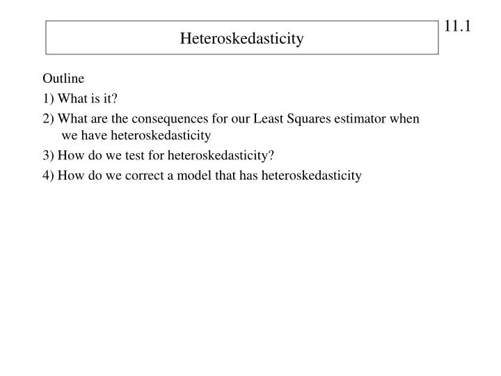
Heteroskedasticity Outline 1) What is it? 2) What are the consequences for our Least Squares estimator when we have heteroskedasticity 3) How do we test for heteroskedasticity? 4) How do we correct a model that has heteroskedasticity
What is Heteroskedasticity Review the assumption of Gauss-Markov • Linear Regression Model y = 1 + 2x + e • Error Term has a mean of zero: E(e) = 0 E(y) = 1 + 2x • Error term has constant variance: Var(e) = E(e2) = 2 • Error term is not correlated with itself (no serial correlation): Cov(ei,ej) = E(eiej) = 0 ij • Data on X are not random and thus are uncorrelated with the error term: Cov(X,e) = E(Xe) = 0 This is the assumption of a homoskedastic error A homoskedastic error is one that has constant variance. A heteroskedastic error is one that has a nonconstant variance. Heteroskedasticity is more commonly a problem for cross-section data sets, although a time-series model can also have a non-constant variance.
This diagram shows a non-constant variance for the error term that appears to increase as X increases. There are other possibilities. In general, any error that has a non-constant variance is heteroskedastic. f(y|x) y . . . x1 x2 x3 x
What are the Implications for Least Squares? We have to ask “where did we used the assumption”? Or “why was the assumption needed in the first place?” We used the assumption in the derivation of the variance formulas for the least squares estimators, b1 and b2. For b2 is was This last step uses the assumption that t2 is a constant 2.
If we don’t make this assumption, then the formula is: Remember: Therefore, if we ignore the problem of a heteroskedastic error and estimate the variance of b2 using the formula on the previous slide, when in fact we should have used the formula directly on this slide, then our estimates of the variance of b2 are wrong. Any hypothesis tests or confidence intervals based on them will be invalid. However, E(b2) = 2 (Verify that the proof of Unbiasedness did not use the assumption of a homoskedastic error.
How do We Test for a Heteroskedastic Error 1) Visual Inspection of the residuals: Because we never observe actual values for the error term, we never know for sure whether it is heteroskecastic or not. However, we can run a least squares regression and examine the residuals to see if they show a pattern consistent with a non- constant variance.
This regression resulted in the following residuals plotted against the variable X (weekly income). What do you see?
2) Formal Tests for Heteroskedasticity (Goldfeld Quandt Test) Many different tests, we will study the Goldfeld Quandt test: a) Examine the residuals and notice that the variance in the residuals appears to be larger for larger values of xt Must make some assumption about the form of the heteroskedasticity (how the variance of etchanges) For the food expenditure problem, the residuals tell us that an increasing function of xt (weekly income) is a good candidate. Other models may have a variance that is a decreasing function of xt or is a function of some variable other than xt.
The Goldfeld Quandt Test: • Sort the data in descending order, and the split the data in half. • Run the regression on each half of the data. • use the SSE from each regression to conduct a formal hypothesis test for heteroskedasticity • If the error is heteroskedastic with a larger variance for the larger values of xt, then we should find: Where: And where SSE1 comes from the the regression using the subset of “large” values of xt., which has t1observations SSE2 comes from the regression using the subset of “small” values of xt, which has t2observations
Conducting the Test: The error is Homoskedastic so that The error is Heteroskedastic It can be shown that the GQ statistic has a F-distribution with (t1-k) d.o.f. in the numerator and (t2-k) d.o.f. in the denominator. If GQ > Fc we reject Ho. We find that the error is heteroskedastic.
Food Expenditure Example: This code sorts the data according to X because we believe that the error variance is increasing in xt. procsortdata=food; bydescending x; data food1; set food; if _n_ <= 20; procreg; bigvalues: model y = x; data food2; set food; if _n_ >= 21; procreg; littlevalues: model y = x; run; This code estimates the model for the first 20 observations, which are the observations with large values of xt. This code estimates the model for the second 20 observations, which are the observations will small values of xt.
The REG Procedure Model: bigvalues Dependent Variable: y Analysis of Variance Sum of Mean Source DF Squares Square F Value Pr > F Model 1 4756.81422 4756.81422 2.08 0.1663 Error 18 41147 2285.93938 Corrected Total 19 45904 Root MSE 47.81150 R-Square 0.1036 Dependent Mean 148.32250 Adj R-Sq 0.0538 Coeff Var 32.23483 Parameter Estimates Parameter Standard Variable DF Estimate Error t Value Pr > |t| Intercept 1 48.17674 70.24191 0.69 0.5015 x 1 0.11767 0.08157 1.44 0.1663 The REG Procedure Model: littlevalues Dependent Variable: y Analysis of Variance Sum of Mean Source DF Squares Square F Value Pr > F Model 1 8370.95124 8370.95124 12.27 0.0025 Error 18 12284 682.45537 Corrected Total 19 20655 Root MSE 26.12385 R-Square 0.4053 Dependent Mean 112.30350 Adj R-Sq 0.3722 Coeff Var 23.26183 Parameter Estimates Parameter Standard Variable DF Estimate Error t Value Pr > |t| Intercept 1 12.93884 28.96658 0.45 0.6604 x 1 0.18234 0.05206 3.50 0.0025 Fc= 2.22 (see SAS) Reject Ho
How Do We Correct for a Heteroskedastic Error? • White Standard Errors: the correct formula for the variance of b2 is: Estimate 2t in the above formula using the squared residual for each observation as the estimate of its variance: This gives us what are called “White’s estimator” of the error variance. In SAS: PROC REG; MODEL Y = X / ACOV; RUN: Food Expenditure example: White standard error: se(b2) = 0.0382 Typical Least Squares: se(b2) = 0.0305
2) Generalized Least Squares Idea: Transform the model with a heteroskedastic error into a model with a homoskedastic error. Then do least squares. Where: Suppose we knew σt. Transform the model by dividing every piece of it by the standard deviation of the error: This model has an error with a constant variance:
2) Generalized Least Squares (con’t) Problem: we don’t know σt. This requires us to assume a specification for the error variance. Let’s assume that the variance increases linearly with xt. Where: Transform the model by dividing every piece of it by the standard deviation of the error.
This new model has an error term that is the original error term divided by the square root of xt. Its variance is constant. • This method is called “Weighted Least Squares”. • More efficient than Least Squares: • Least Squares gives equal weight to all observations. • Weighted Least Squares gives each observation a weight that is inversely related to its value of the square root of xt large values of xt which we have assumed have a large variance will get less weight than smaller values of xt when estimating the intercept and slope of the regression line
We need to estimate this model: This requires us to construct 3 new variables: We estimate this model: Notice that it doesn’t have an intercept
SAS code to do Weighted Least Squares: ystar = y/sqrt(x); x1star = 1/sqrt(x); x2star = x/sqrt(x); procreg; foodgls:model ystar=x1star x2star/noint; run;