Acoustic Wave Equations: Hooke's Law, Newton's Law, and Solutions

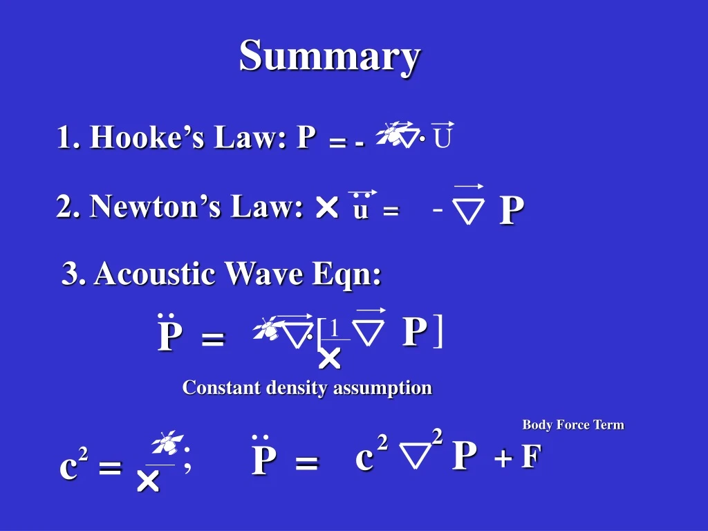
1. Summary .. .. P - k r k ] u = P - [ 1. Hooke’s Law: P P = = - U 1 r 2. Newton’s Law: 3. Acoustic Wave Eqn: k c = 2 r .. 2 P c ; P = 2 Constant density assumption Body Force Term + F

2. Solutions to the Acoustic Wave Equation

3. Outline • Plane Wave: Dispersion relationship, freq., wavelength, wavenumber, slowness, apparent velocity, apparent wavelength. 2. Spherical Wave. 3. Green’s function, asymptotic Green’s function.

4. Harmonic Motion: w=2pi/T T = sec/cycle Phase P = Acos(wt) Period Time (s) 1/T=f = cycle/s 2pi/T=w=radians/s

5. Harmonic Ripples: k=2pi/ Phase P = Acos(kx) Wavenumber Time (s) Wavelength x

6. Harmonic Ripples: k=2pi/ Phase P = Acos(kx) Time (s) Wavenumber Wavelength x

7. Plane Wave Solution (1) Phase=O (2) i(kx-wt) P = Ae k 2 2 wavenumber (k - w ) P = 0 angular frequency k = w c = k = w = 2 pi 2 c c 2 r c .. 2 P c ; P = 2 dO = kdx/dt –w =0 dt dx/dt =w/k Faster Velocities = Stiffer Rocks Plug (2) into (1) [class exercise] k & w no longer independent Variables if dx/dt is a constant Dipsersion relation Wavefront = Line of constant phase Wavelength=shortest distance between adjacent peaks

8. Dispersion Relation w l dx c = = = T k dt This says: a hamonic wave propagates one wavelength in one period

9. Outline • Plane Wave: Dispersion relationship, freq., wavelength, wavenumber, slowness, 2D apparent velocity, 2D apparent wavelength. 2. Spherical Wave. 3. Green’s function, asymptotic Green’s function.

10. k*r describes a straight line with k perpendicularto line i(k r - wt) (2) = Ae = |r||k| cos(O) k = constant Any pt along line phase is cnst O k r r z kis perpendicular to wavefront i(k x + k z - wt) P = Ae x z x (x,z)

11. 2D Plane Wave Solution i(k r - wt) (2) = Ae Equation of a line: k r = cnst k = (k , k ) = |k|(sin , cos ) x z k Phase i(k x + k z - wt) P = Ae x z

12. 2D Plane Wave Solution = = cosO sinO i(k r - wt) (2) = Ae Equation of a line: k r = cnst k = (k , k ) = |k|(sin , cos ) x z k k = 2pi/|k| z x z Phase i(k x + k z - wt) P = Ae x z

13. Apparent Velocity dz/dt=apparent V dx/dt=apparent V = = z x x z T T sinO = T z x Time (s)

14. Examples: dx/dt = v/sinO Examples: dx/dt = v/sinO=v = = O=90 z x Time (s)

15. Examples: dx/dt = v/sinO = = = O=0 z x Time (s)

16. Marine Experiment

17. X (ft) 250 0 0.45 Each arrival type has different apparent x-velocity w/r to x Time (s) Reflection Refraction Direct 0.0 Direct Reflection Refraction

18. x x 2 2 X (ft) 250 0 0.45 Each arrival type has different apparent x-velocity w/r to x Refraction Time (s) Reflection Direct 0.0 Direct Critical angle Refraction Reflection Or Head Wave

19. Outline • Plane Wave: Dispersion relationship, freq., wavelength, wavenumber, slowness, apparent velocity, apparent wavelength. 2. Spherical Wave. 3. Green’s function, asymptotic Green’s function.

20. Recall: Work on a Spring du dW = -Fdu=-kudu W = Fdu spring Work Performed: Mechanical work=amount energy transferred by a force acting through distance W = dW = -k udu = -ku /2 2

21. Energy of an Acoustic Wave du F=Pdzdy W =- (Pdzdy)du =- PdV 2 = P V W = PdP V k 2 k dy Work Performed: dz Mechanicalwork=amount energy transferred by a force acting through distance dx dW = -(Pdzdy)du = -PdV but dV = -VdP/k Hooke’s Law Energy proportional to amplitude squared

22. Outline • Plane Wave: Dispersion relationship, freq., wavelength, wavenumber, slowness, apparent velocity, apparent wavelength. 2. Spherical Wave. 3. Green’s function, asymptotic Green’s function.

23. Spherical Wave in Homogeneous Medium i(k r - wt) (2) Ae satisfies P = r except at origin Geometrical speading Phase change perp. to circles .. 2 2 2 r = x + y + z 1 2 P c P = 2 2 3 4 Ray is traced such that it is always Perpendicular to wavefront r r is distance between pt source and observer at (x,y,z)

24. Spherical Wave in Homogeneous Medium i(k r - wt) (2) Ae satisfies f = r except at origin Phase change perp. to circles .. 2 f c f = 2 (2) (1) 2 f (3) Class Exercise: Plug (1) into (2), then plug result into (3) to show it is satisfied everywhere except origin

25. g(x,t |x ,t )= s s o Propagation time { Listening time Listening & source coords. 1 t=|r|/c (t-|r|/c) = 0 |r| ottherwise Geometrical Spreading 2 2 2 |r| = x + y + z Propagation time = c c What is a Green’s Function? Answer: Point Src. Response of Medium Answer: ImpulsePoint Src. Response of Medium

26. { 2 2 + k [ ] G(A|x) =- (x-A); 1 t-t =|r|/c (t -|r|/c) = s |r| |r| g(x,t|x ,0 ) = s 0 ottherwise Fourier iwr/c e G(x|x ) = s p 4 What is a Green’s Function? Answer: Point Src. Response of Medium Answer: Impulse-Point Src. Response of Medium

27. { 1 t-t =-|r|/c (t+|r|/c) = s a |r| |r| g(x,t|x ,0 ) = s 0 ottherwise Fourier -iwr/c a e G(x|x ) = s 2 2 + k [ ] G*(A|x) =- (x-A); p 4 What is an Acausal Green’s Function? Answer: Point Src. Response of Medium Answer: Acausal Impulse-Point Src. Response of Medium g(x,-t|x ,0 ) = G(x|x )* =

28. { Listening time Listening & source coords. 1 t=-|r|/c (t+|r|/c) = 0 |r| ottherwise Geometrical Spreading r t=-1 t=-2 t=-3 2 2 2 |r| = x + y + z Propagation time = c t=-4 c What is an Acausal Green’s Function? Answer: Point Src. Response of Medium Answer: Impulse-Point Src. Response of Medium

29. { 1 t-t =|r|/c (t -|r|/c) = s |r| |r| |r| |r| g(x,t|x ,0 ) = s 0 ottherwise derivative Fourier ~ d iwr/c e G(x|x ) = iw/c s 2 + O(1/r ) dr n n r iwr/c e G(x|x ) = iw/c s 2 + O(1/r ) What is a Green’s Function? Answer: Point Src. Response of Medium Answer: Impulse-Point Src. Response of Medium ~ iwr/c e G(x|x ) = s Far field approx k

30. What is a 2D Green’s Function?

31. Wave in Heterogeneous Medium i(wt - wt) G = Ae satisfies except at origin Geometrical speading w i i i i i i i Total time i Time taken along ray segment .. 1 2 G c G = 2 2 3 4 (2) kr = (kc ) r /c = wt r r i Valid at high w and smooth media

32. = G(x |x ) s |r| What is Reciprocity? iwr/c e G(x|x ) = s x x s

33. G(x|x ) = s = G(x |x ) = G(x |x ) s s |r| What is Reciprocity? Interchanging src & rec does not change value of r=|x – x| iwr/c e G(x|x ) = s x x s

34. g(x,t|x ,ts) g(xs,-ts|x,-t ) = g(x,t-t |x ,0 ) g(x,t-t |x ,0 ) s s s s |r| { 1 t - t=|r|/c (t – t -|r|/c) = s g(x,t|x ,t ) = g(x,t|x ,t ) = s s s s s 0 ottherwise x x s What is Stationarity? Stationarity Reciprocity Observed wave depends on difference between observation and start times, not on absolute start time

35. a G(B|x) = G(B|x)* 1. g(x,t|x ,ts) g(xs,-ts|x,-t ) = g(x,t-t |x ,0 ) s s i(wt - wt) G(B|x) = 2. Ae G(x|x ) = G(x |x ) s Bx s g(x,t|x ,t ) = s s x x 3. s x x s = Summary Causal & Acausal GF Source vs Sink Heterogeneous Hi-freq. Green’s function Reciprocity 4. Stationarity s

36. Exercises

37. Define Ricker and model variables Modeling MATLAB Exercise % twod.m computes forward model of 2-layer model and % % --^----x-----------A------------B------ % | % d v1 % | % -v------------------------------------ % % v2 % % Define 2-layer model: % d - input - depth of layer % (v1,v2) - input- velocities top/bottom layers % (dx, L) - input- src-geo (interval, recording aperture) %(np,fr,dt) –input -(# pts wavelet, peak frequency, time interval) clear all % Model input variables v1=1.0;v2=2.0;d=.2725;L=1;dx=.005;x=[0:dx:L];nx=round(length(x)); np=100;dt=.006;fr=15; % Define Ricker Wavelet [rick]=ricker(np,dt,fr); % Compute synthetic seismograms 2-Layer model figure(1);[seismo,ntime]=forward(v1,v2,dx,nx,d,dt,np,rick,x,fr); % Correlate G(A|x) and G(B|x) and sum over x % to get G(A|B) figure(2);A=round(nx/3);B=round(nx/2); [GABT,GAB,peak]=corrsum(ntime,seismo,A,B,rick,nx);

38. Loop over srcs Loop over recs Compute traveltimes of primaries & multiples Seismogram calculation MATLAB Exercise function [seismo,ntime]=forward(v1,v2,dx,nx,d,dt,np,rick,x,fr) r=(v2-v1)/(v2+v1);r1=r*r;r2=r1*r; for ixs=1:nx % Loop over sources xs=(ixs-1)*dx; t=round(sqrt((xs-x).^2+(2*d)^2)/v1/dt)+1; %Primary Time t1=round(sqrt((xs-x).^2+(4*d)^2)/v1/dt)+1; %1st Multiple Time t2=round(sqrt((xs-x).^2+(6*d)^2)/v1/dt)+1; %2nd Multiple Time s=zeros(nx,ntime); for i=1:nx; % Loop over recievers s(i,round(t(i)))=r/t(i); %Primary s(i,round(t1(i)))=-r1/t1(i); % 1st-order Multiple s(i,round(t2(i)))=r2/t2(i); % 2nd-order Multiple ss=conv(s(i,:),rick); % Convolve Ricker & Trace s(i,:)=ss(1:ntime); % Synthetic Seismograms seismo(ixs,i,1:ntime)=ss(1:ntime); end c=seismo(ixs,:,:);c=reshape(c,nx,ntime); imagesc([1:nx]*dx,[1:ntime]*dt,c');xlabel('X(km)');ylabel('Time (s)') title('Shot Gather for Two-Layer Model') pause(.1) end Display CSG

39. Summary t Period

40. Summary 1. V = T k 2. k=|k|(sin O, cos O) i(kx-wt) P = Ae O k = r Wave motion Rock stress-strain ; = = z x cos O sin O ; V = V = x z x z T T

41. x 2 Summary p Slowness Vector 3. k=|k|(sin O, cos O) = p w w 4. Geophone sampling: Avoid Spatial aliasing X < x 2 1/c P ~ ikP implies particle motion || propagation direction Geophone sampling interval

42. Spherical Wave in Homogeneous Medium i(k r - wt) (2) Ae satisfies f = r except at origin Phase change perp. to circles .. 2 f c f = 2 (2) (1) 2 f (3) Class Exercise: Plug (1) into (2), then plug result into (3) to show it is satisfied everywhere except origin

43. x x 2 2 250 Eyeball estimation Apparent Velocity 0 0.45 Each arrival type has different apparent x-velocity w/r to x Refraction Time (s) Reflection Direct 0.0 Direct Critical angle Refraction Reflection Or Head Wave

44. Summary t =c =c t dx/dt =2w/2k dx/dt = w/k x x w w/k=c k Dispersionless medium c independent w Typically true for body waves at seismic w t Implication: Wavelet shape not distorted as wave propagates x 5. Dispersionless velocity: c = w/k = group velocity = dx/dt

45. Summary t =c dx/dt = w/k x dispersion: group dw/dk = phase c w No dispersion: group dw/dk = phase c w dw/dk = c(w) = w/k dw/dk = c(w) = w/k k k Warning: Attenuation destroys high frequencies at large offsets and so wavelet shape distorted. This is not dispersion. In practice w vs k curves by FFT d(x,t). Can be Used to get shear velocity distribution for statics. dw(k )/dk = dw(k )/dk 2 1 6. Dispersion phase velocity: c(w) = w/k(w) w=4pi/T w=2p/T dx/dt =2w/k(2w) t =c(w) x Group velocity dw/dk not equal phase velocity w/k Typically true for surface waves at seismic w cone t Implication: Wavelet shape distorted w/r x x

46. Summary t =c dx/dt = w/k x 6. Dispersion phase velocity: c(w) = w/k(w) w=4pi/T w=2p/T dx/dt =2w/k(2w) t =c(w) x

47. data 0 Time (s) 2.0 Receiver (m) 0 3600 The original data from Saudi cone

48. 0 0 Time (s) Time (s) 2.0 2.0 Receiver (m) 0 Receiver (m) 0 3600 3600 The removed: F-K VS NLF+Interferometry

49. 0 0 Time (s) Time (s) 4.0 4.0 0 0 Receiver (m) 5000 Receiver (m) 5000 Line12 before & after removing surface waves

50. 0 0 Time (s) Time (s) 2.0 2.0 Receiver (m) 0 Receiver (m) 0 3600 3600 Data from Saudi reflections reflections reflections Surface wave cone