Download
1 / 28
280 likes | 435 Views
Struttura dei materiali al calcolatore: Idee di base, capacità di calcolo, approssimazioni e qualche applicazione (ENEA, 18 novembre 2003). Carlo Massobrio Institut de Physique et Chimie des Matériaux de Strasbourg (IPCMS) 23 Rue du Loess BP 43 F-67034 Strasbourg Cedex 2, France.

E N D
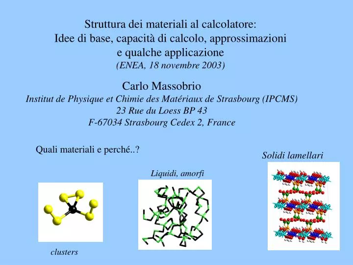
Struttura dei materiali al calcolatore: Idee di base, capacità di calcolo, approssimazioni e qualche applicazione (ENEA, 18 novembre 2003) Carlo Massobrio Institut de Physique et Chimie des Matériaux de Strasbourg (IPCMS) 23 Rue du Loess BP 43 F-67034 Strasbourg Cedex 2, France Quali materiali e perché..? Solidi lamellari Liquidi, amorfi clusters
Questo non é un panorama dell’IPCMS ma bensí del quartiere Petite France di Strasburgo…!!! L’IPCMS si interessa alla sintesi e alla caratterizzazione di NUOVI materiali NUOVI: creati a partire da nanostrutture e modificati via inserzione di nuovi componenti: non si sa a priori DOVE sono gli atomi..!!! Conti su scala atomica: complemento indispensabile agli esperimenti Scala atomica = ogni atomo e’ descritto dal campo di forze degli altri
Scienza dei materiali computazionale Dinamica molecolare ab-initio Idea: Sistema dinamico "esteso " Gradi di libertà: ioni + funzioni d’onda Evoluzione adiabatica = elettroni vicini allo stato fondamentale La struttura elettronica e’nota per ogni posizione (e evolve in funzione della temperatura) Dettagli pratici Base di Onde Piane (structura periodica) Pseudopotenziali (interazione tra il core e gli elettroni di valenza) Quadro teorico : funzionale della densità (DFT) (teoria elettronica a 1 corpo)
Quali approssimazioni…? La DFT non é una teoria esatta: secondo l’ipotesi di Kohn et Sham gli elettroni sono innanzitutto degli oggetti indipendenti, con gli effetti di correlazione introdotti a posteriori La descrizione del legame chimico dipende fortemente dalla funzionale di scambio e correlazione usata: vedi esempio del liquido GeSe2 Benché sufficiente nella maggior parte dei casi (il volume diventa un sistema periodico) Il numero di gradi di libertà e’ limitato (100-1000)
Che calcolatori e programmi usiamo e con quali prestazioni..?? (1) Codice cpv : scritto da Alfredo Pasquarello (EPFL, Lausanne), vettoriale, facile da capire, modificare e usare. Stile di impiego: utilizzatore conscio dei limiti delle "scatole nere“ Calcolatore NEC SX5 (centro di calcolo nazionale IDRIS) Esempio: GeSe2 amorfo, 120 atomi Memory Size: 3900 MB 92154 onde piane, un passo = 28 s.3323 MFLOPS Per fare 1 ps: 14 ore CPU, con 4200 ore: 300 ps (3.10-10 s) Attenzione: 120 atomi e’ il minimo sistema compatibile con uno studio di correlazioni spaziali oltre i primi vicini..!!!
Che calcolatori e programmi usiamo e con quali prestazioni..?? (2) Codice cpmd : scritto dal gruppo di Michele Parrinello (IBM Zürich, Max Planck Stuttgart, ETH Zürich) : parallelo, ben documentato, gestito da un consorzio, permette una produzione di risultati su scala “industriale”: “scatola nera” moderna, accessibile e affidabile Calcolatore disponibile in Montpellier (un altro simile trovasi in Orsay): IBM SP 29 nodi SMP(NHZ) a 16 processori, 464 processori Power3+, 16 Gbytes/nodo, Prestazioni: 1 Teraflop Esempio: Cu2(OH)3(CH3COO) solido, 72 atomi 249775 onde piane, un passo = 12 s.su 48 processori Memory Size ~ 5000 MB Problema: il rilassamento delle posizioni atomiche non é "immediato“ (puo’ richiedere migliaia di iterazioni)
Understanding molecular-based magnetic materials via a DFT-plane waves approach Outline: Hybrid organic-inorganic materials: transition metal hydroxides Why DFT with plane waves (and pseudopotentials)..? Test cases of accuracy (molecular complexes) Application to large systems
Acknowledgments Eliseo Ruiz (Barcelona) calculations with Gaussian Mauro Boero (Tsukuba, Japan) assistance with pseudopotentials Experimental counterpart : M. Drillon, P. Rabu (IPCMS) Resources: IDRIS computer center Orsay CINES computer center Montpellier
Hydroxide based organic -inorganic magnets Mn , Co, Ni , Cu
Peculiar behavior of susceptibility Precursor of Layered Hybrid Magnetic Materials Cf. Advanced Materials 10, 1024 (1998)
Our purposes optimize the geometries of large structures insight into magneto-structural correlations Manageable scheme:DFT + Pseudopotentials + plane waves Accurate forces for minima search Open issue: accuracy of calculated exchange couplings J "Lower bound" for DFT + Pseudopotentials + plane waves 0.01-0.02 eV (80-150 cm-1) This is close to typical exchange couplings..!!! Open issue: is the approach reliable for molecular magnetism..??
Methodology Selected homodinuclear Cu complexes in a periodic box, V=L3 J= E(S=0) - E(S=1) L= 35 a.u. (no changes in J for larger boxes) Energy cutoff Rc= 90 Ry (no changes in J for larger cutoffs) Converged calculation parameters Computational effort for each E 2.4X10⁶ plane waves for the density 5 hours, 48 pr. of SP4
Copper (II) acetate from Electronic Structure and Magnetic Behavior in Polynuclear Transition-metal Compounds, in Magnetism; Molecules to Materials II E. Ruiz et al., 2001, p.227 (Wiley VCH) Method J (cm-1) Exp. -297 DDCI-2 -77 DDCI-3 -224 CASSCF -24 CASPT2 -117 UHF-bs -27 Xa-bs -848 SVWN-bs -1057 B3LYP-bs -299 BLYP-bs -779 BLYP (this work) J = -518cm-1
See E. Ruiz et al., (Gaussian) J. of Comp. Chem. 20, 1391 (1999) [Cu2(m-OH)2(bipym)2](NO3)2 Exp. J = 114 cm-1 B3LYP J = 113 cm-1 BLYP J = 221 cm-1 BLYP (this work) J = 95 cm-1
B3LYP J = 56 cm-1 BLYP J = 100 cm-1 [(dpt)Cu(m-Cl)2Cu(dpt)]Cl2 dpt= dipropylenetriamine Exp. J = 42.9 cm-1 (M. Rodríguez et al., Inorg. Chem. 1999, 38, 2328) E.Ruiz (Gaussian) BLYP (this work) J = 61 cm-1
Benchmarks calculations on homodinuclear Cu(II) complexes Good performances of plane waves pseudopotential schemes Exp, B3LYP (Gaussian) BLYP (plane waves) BLYP (Gaussian) J
DFT-plane waves-pseudopotentials for molecular magnetic materials FOR AGAINST Optimization of structures: large "new materials" treated self-consistently Good performances for molecules High cost Not all functionals yet implemented (B3LYP..?) Control of initial spin densities distributions not straightforward Less suited for charged systems
Calculations on solid-state compounds Cu2(OH)3NO3 ELF Spin densities
Peculiar behavior of susceptibility Precursor of Layered Hybrid Magnetic Materials Cf. Advanced Materials 10, 1024 (1998)
DFT calculations (first principles molecular dynamics) Plane wave (PW) basis set + pseudopotentials GS Kohn-Sham approach + GGA i GGA GS = ground state for both electrons and ions Total spin fixed S=0 Collinear case Nat = 48, 96, 144 (i.e. 8, 16, 24 Cu atoms) PW Energy cutoff = 90 Ry electron density spin density X-ray diffraction electron densities From the structure factors to the atomic electron densities + deformation densities (chemical bonding) cf. P. Coppens, X-ray charge densities and chemical bonding (Oxford Science, 1997)
Theory vs X-ray diffraction models DFT X-ray: Spherical model X-ray: Multipole model
J a Cu O a Molecular models: advantages and limitations Four exchange pathways Cu-O-Cu in the plane (Cu2(OH)3NO3) layers Shortest Cu-O distances: J2 and J3 (both O OH groups) J2 In hydroxo and alkoxo-bridged molecular Cu(II) compounds J4 J1 J3 Cu2 Cu1 Cu1 What is missing..??? Interplanar interactions cf. Electronic Structure and Magnetic Behavior in Polynuclear Transition Metal Compounds, E.Ruiz et al (From Molecules To Materials, Miller, Drillon eds., Wiley). 3d magnetic character..?
Interplanar interactions DFT: Electron localization function (ELF) Electron density (X-ray)
0.001 a.u. 0.08 a.u. 0.01 a.u. Spin density between the layers
X-ray electronic densities along the exchange pathways J2 and J3 expected to be more effective J2 J1 Cu1- Cu1 Cu2 - Cu2 J3 J4 Cu1 - Cu2 Cu1- Cu2
0.006 a.u 0.06 a.u Spin densities (slices) N= 96 (2X1Y2Z) Spin structure: Frustration effects Correlations Cu2-Cu1-Cu2 N= 96 (2X2Y1Z)
A B |J1| 25 K, J1= -J2 EXP: About the estimate of the exchange couplings J Ising spin Hamiltonian We look for all possible spin structures compatible with S=0 (interplanar interactions only) To be determined : J1, J2, J3, J4 EA - EB 100 K |J2|, 50-100 K, J2= -J3