Download
1 / 37
370 likes | 550 Views
Integer Optimization. Summer 2013. Integer Optimization. In integer optimization, at least one variable is restricted to integer values. But the decision variables can be linear and / or nonlinear. We will consider only linear variables. Linear Optimization Classification.

E N D
Integer Optimization Summer 2013 Integer_LP
Integer Optimization In integer optimization, at least one variable is restricted to integer values. But the decision variables can be linear and / or nonlinear. We will consider only linear variables. Linear Optimization Classification Within ILP, we can have either “all integer” or “mixed integer” model. A variable restricted to 0 or 1 values is called a binary variable. Solver can solve all ILP models but it takes longer compared to the LP model without integer restriction. Solver can also be used for many nonlinear optimization models. Integer_LP
LP example What if x1and x2 must be integers? We can try four closest points. 3 2 1 x1= 0.00, x2 = 2.05 LP optimal: Z = 16.80 x1= 2.00, x2 = 1.85 (1, 2), (2, 2) are infeasible. At (1, 1), Z = 9 . At (2, 1) , Z = 10 Integer optimal : (0, 2), Z = 16! 1 2 3 4 X1 Optimal may not be a corner point Integer_LP
9 8 7 6 5 4 3 2 1 1 2 3 4 5 6 7 8 9 A simple LP example Optimal LP: x1= 3.125, x2 = 2.875 with Z = 53.5 Optimal ILP: x1= 1, x2 = 4 with Z = 51 Many approaches: Start with LP. Cutting Plane: Add one constraint at a time till you get an optimal solution. Branch and Bound: If the current solution is not integer, split the problem into two problems (with one constraint added to each) and solve again. Repeat till you get integer optimal solution. Solver uses this approach. …. There is no efficient procedure (like Simplex) available to find the optimal solution. Integer_LP
9 8 7 6 5 4 3 2 1 1 2 3 4 5 6 7 8 9 ILP: B&B Start with the LP solution. Add two branches with extra constraints if there is a non-integer value and solve the two sub-problems. LP: Z = 53.5. (3.125, 2.875) x2 ≥ 3 x2 ≤ 2 Z = 50. (4, 2) Z = 53.222 (2.889, 3) x2 ≥ 3 Feasible! No need to expand this branch. This is a lower bound. Add two branches x2 ≤ 2 Integer_LP
9 8 7 6 5 4 3 2 1 1 2 3 4 5 6 7 8 9 ILP: B&B Start with the LP solution. Add two branches with extra constraints if there is a non-integer value and solve the two sub-problems. LP: Z = 53.5. (3.125, 2.875) x2 ≥ 3 x2 ≤ 2 Z = 50. (4, 2) Z = 53.222 (2.889, 3) x2 ≥ 3 Feasible! No need to expand this branch. This is a lower bound. Add two branches x2 ≤ 2 Integer_LP
Branch and bound methodology Root node LP: Z = 53.5 (3.125, 2.875) B & B methodology can be applied to many other problems besides ILP. x2 ≤ 2 x2 ≥ 3 Z = 50 (4, 2) Z = 52.222 (2.889, 3) x1 ≤ 2 x2 ≤ 3 x1 ≥ 3 x2 ≥ 4 Excel solver uses B & B methodology. Infeasible! Z = 52.176 (2, 3.47059) Optimum! Z = 51. (1, 4) Z = 47. (2, 3) Integer_LP
ILP with Solver using B&B: Some comments In large ILP problems, there may be thousands of branches for exploration. Solver has to solve thousands of LP problems and this can be very time consuming. We can curtail this by selecting appropriate options. Enter everything and click on the Options. Integer_LP
Selecting appropriate values, we can terminate the program earlier and accept the best result obtained up to the termination time. This may or may not be optimal. Integer_LP
Integer Linear Programming models We will look at examples. Integer_LP
Knapsack problem You want to fill your knapsack with different items to maximum value of the goods you are carrying. There are n types of items and there is a weight limit. Formulation: Let there be n different item. For item k, let Wk to denote weight per unit and Vk denote the value per unit. Let B be the maximum weight you can carry. We will use yk to denote number of units of item k included in the knapsack. Maximize V1 y1 + V2 y2 + … +Vnyn Subject to: W1 y1 + W2 y2 + … +Wnyn≤ B y1 , y2 , …, yn 0 and integer So many different versions of the problem exist that a book (with over 400 pages) has been published. We will consider two versions. Version 1: variables y can take only binary values. Version 2: equality constraint and minimization objective function. Integer_LP
Version 1: Capital Budgeting Assume budget (B) = 176 million dollars. Which projects should we select to maximize Net Present Value (NPV)? Maximize 10 y1 + 17 y2 + 16 y3 + 8 y4 +14 y5 Subject to: 48 y1 + 96 y2 + 80 y3 + 32 y4 +64 y5 ≤ 176 y1 , y2 , y3 , y4, y5 all binary (0 or 1). Integer_LP
Capital Budgeting Example Any problems with the model? Integer_LP
Knapsack problem – Version 2 Minimize V1 y1 + V2 y2 + … +Vnyn Subject to: W1 y1 + W2 y2 + … +Wnyn= B, y1 , y2 , ynall integers 0n Minimize with equality constraint Recognize these examples? Ex 1: Min. y1 + y2+ y3 + y4+ y5 = Z Subject to: y1 + 5 y2+ 10 y3 + 0 y4+ 25 y4= 42 y1 , y2 , y3 , y4, y5all integers 0 Solution: y1 = 2, y2 = 1, y3 = 1, y4 = 0, y5 = 1, Z = 5 Ex 2: Min. y1 + y2+ y3 + y4+ y5 = Z Subject to: y1 + 5 y2+ 10 y3 + 20 y4+ 25 y4= 42 y1 , y2 , y3 , y4, y5 all integers 0 Solution:y1 = 2, y2 = 0, y3 = 0, y4 = 2, y5 = 0, Z = 4 Integer_LP
S2 Set Covering problem D1 * S1 D9 * S3 S7 Nine districts (D1, D2,.., D9) are to be covered within acceptable time limits by emergency vehicles. D2 * S4 S6 S5 D8 * Sevenpotential sites (S1, S2, …, S7) have been identified. D3 * D4 * D7 * Each site can reach only some districts within the time limit. D6 * D5 * We need to cover all districts with minimum number of sites. Integer_LP
Set Covering problem Nine districts (D1, D2, , D9) are to be covered within acceptable time limits by emergency vehicles. Seven sites (S1, S2, …, S7) have been identified. Each site can reach only some districts within the time limit. We need to cover all districts with minimum number of sites. What do 0 and 1 in the table indicate? Integer_LP
Set Covering Formulation Integer_LP
Set Covering Solution There may be alternate optimum solutions. Integer_LP
Binary Variables & Logical Relationships In many models, one or more constraints involving binary variables can be added to satisfy desired logical relationship. Suppose we have several projects P1 , P2, P3, etc. and we define binary variables Y1, Y2, Y3, etc. Y1 = 0 means project P1 is not selected Y2 = 1 means project P2 is selected and so on. We need to add constraint(s) such that when the relationship is satisfied, all constraints must be met and when the relationship is not satisfied, at least one of the constraint must fail. Suppose the logical relation is: Select P2 or P5 or both. We need only one constraint. Y2+Y5 1. We will explain this on the next slide. Integer_LP
Select P2 or P5, or both. Y2 + Y5 ≥ 1 If only P2 is selected, Y2 = 1. If only P5 is selected, Y5 = 1. If P2, P5 selected, Y2+Y5 = 2 but when both are not selected, Y2+Y5 = 0 and the constraint is not satisfied. Select at most one project from P3 , P4 , P5. Y3 + Y4 + Y5 ≤ 1 If 0 or 1 projects are selected, the constraint is satisfied. If two are selected, Y3+Y4 +Y5 will be equal to 2 and the constraint is not satisfied. Same if you select all three. If P5 is selected, then P4 must be as well. Y4 - Y5 0 If P5 is selected, Y5 = 1 then Y4 must also be 1. If Y5=0, Y4 can be 0 or 1. If Y5 =1 and Y4 = 0, the constraint is not satisfied. Integer_LP
Linking Constraints and Fixed Costs Suppose we purchase x units of a product at unit cost C. For sending the purchase order, there is a fixed cost F. So the total purchase cost will be (F + Cx). If this value is included in the objective function, then we will end up with fixed cost F even when x = 0. This should not happen. There should be no fixed cost when we don’t buy. To correct this, we introduce a binary variable y and add a new constraint as follows. Minimize Fy + Cx Subject to: x ≤ My where M is a large number. y = 0 or 1 Note that when x = 0, y can be 0 or 1 according to the first constraint and minimization will force it to zero. When x > 0, y will be forced to a value of 1. Integer_LP
Dynamic Lot Sizing Model • The model assumptions / requirements are as follows. • We have a single product with demand D1, D2, …, Dn for n periods (periods P1, P2, … , Pn). • Decision variables: X1, X2, …, Xn. These can be production or purchase quantities, called lot sizes. • No shortages are allowed. • There are no capacity constraints. • There is a fixed setup cost (sometimes called ordering cost) K1, K2, …, Kn. • For inventory left over at the end of each period, there is a per unit holding cost H1, H2, …, Hn. • The unit production (or purchase) cost is C1, C2, …, Cn. . This is similar to the production planning model except for the fixed setup cost K. This means we need extra binary variables. Integer_LP
Lot sizing formulation (shown for 3 periods) X1 X2 X3 Let X1, X , X3 be quantities ordered in P1, P2, P3 D1 D2 D3 I1 I2 I3 Minimize Z = C1X1 + C2X2 + C3X3 + K1y1 + K2y2 + K3y3 + H1I1 + H2I2 + H3I3 Subject to: X1 , X2 , X3≥ 0 I1 , I2 , I3≥ 0 X1 - My1 ≤ 0 X2 - My2 ≤ 0M is a very large number X3 - My3 ≤ 0 y1 , y2 and y3 : 0 or 1 Integer_LP
Lot sizing model: Procedure when per unit purchase price does not change. In period 1, we must buy at least 87 units. Why? In period 1, we could buy 87, 88, 89, …., 376 or 377 units. Why? Property: We should not buy units equal to partial period demand. We should buy 87 or 87+50 or 87+50+100, an so on In P1 Buy 0 or 50 or 50+100 , …., 50+100+60+80 In P2. Why? Integer_LP
Lot sizing model: We will calculate costs of several alternatives. What does cell P2-P4 indicate? Buying (50+100+60) units to meet demand for periods P2 to P4. Integer_LP
We will do calculations column by column from top to bottom. Integer_LP
0 120 0 120 0 120 65 185 0 120 335 455 Best cost for P3 occurs in row P3. We don’t need to calculate numbers here. 120 125 0 245 120 125 140 385 120 185 130 0 315 185 315 Integer_LP
185 130 323 638 185 130 87 402 315 135 0 450 315 135 120 570 How to read the solution? 402 138 0 540 402 540 Integer_LP
Buy in period 5 for period 5 (80 units) • Total cost = $540 • Buy in period 3 for periods 3 & 4 (160 units) • Buy in period 1 for periods 1 & 2 (137 units) Integer_LP
What numbers will go in the box for row P3, column P5 (buying in period 3 for P3, P4 and P5)? Integer_LP
Excel solution Ordering policy Total cost Integer_LP
Aggregate Planning Suppose 1 pickup = 1.6 cars Objective:to develop a feasible production plan on an aggregate level based on demand, capacities, costs and other factors. • 500 pickups and 1600 cars equivalent to: • (500 * 1.6) + 1600 = 2400 cars, or • 500 + (1600 / 1.6) = 1500 pickups. How is equivalence determined? Integer_LP
Calculate aggregate demand in term of the standard product “CC”. 1.5 * 2400 / 2.0 = 1800 3.0 * 1000 / 2.0 = 1500 2.0 * 2000 / 2.0 = 2000 1.0 * 1200 / 2.0 = 600 5900 What to do if capacity in standard units is 5000? What if demand remains high (or low) month after month? Integer_LP
Developing Aggregate Plan. For aggregate planning, the planned period is called the planning horizon. For planning, we can use different strategies: Chase, Level or a combination. Chase Strategy: produce quantity equal to aggregate demand for each period (to keep inventory level zero). Level Strategy:Produce quantity equal to the average requirement over the planning horizon. • Policies (constraint) examples: • Capacity in each period may be limited. • No shortages may be permitted (customer satisfaction). • No inventory is kept. • Must leave certain inventory at the end of period X. • Overtime limited to 20% of regular time. • Hiring and firing of workers. Sometime we may have soft constraints. We try to meet these constraints as much as possible. LP does not use soft constraints. Integer_LP
Aggregate Planning Model(for 12 periods) • Periods: P1, P2, .., P12 • Aggregate demand D1, D2, ..,D12 • Production: X1, X2, ..., X12 • End inventory: I0, I1, I2, .., I12. • Regular workers: R0, R1, R2, ..,R12 • Overtime O0, O1, O2, ..,O12 • Ik = Ik-1 + Xk– Dk • If Ik> 0 we have to pay holding cost on inventory. • If Ik< 0 we have to pay shortage cost on demand not met. R0, O0 R1, O1 R2, O2 R3, O3 Workers X1 X2 X3 Production I0 I1 I2 I3 D1 D2 D3 Demand • A worker make units in a day. The worker makes units in overtime (overtime is less than a day). Integer_LP
Chase Strategy Level Strategy • No inventory. • You can hire or lay off workers (some cost involved). Overtime cannot be given to new workers. • Level production (shortages permitted ) • Constant workforce (hire or lay off only in P1) To find the minimum cost production plan. Cost = Regular wage & benefit + Overtime wage & benefit + Cost of hiring + Cost of lay off + Holding cost + Shortage cost Other costs remain fixed during the year. What are the decision variables for each strategy? How to handle holding / shortage cost for the level strategy? Integer_LP
Capital Budgeting Example Reduce the budget to 175. Integer_LP