Download
1 / 64
1.21k likes | 2.4k Views
Chapter 7 Wavelets and Multiresolution Processing. An example. The Welch periodogram of this speech signal. Stationary analysis is only applicable to stationary signals. Non-stationary signals require analysis techniques that encompass time variation the short-time Fourier transform

E N D
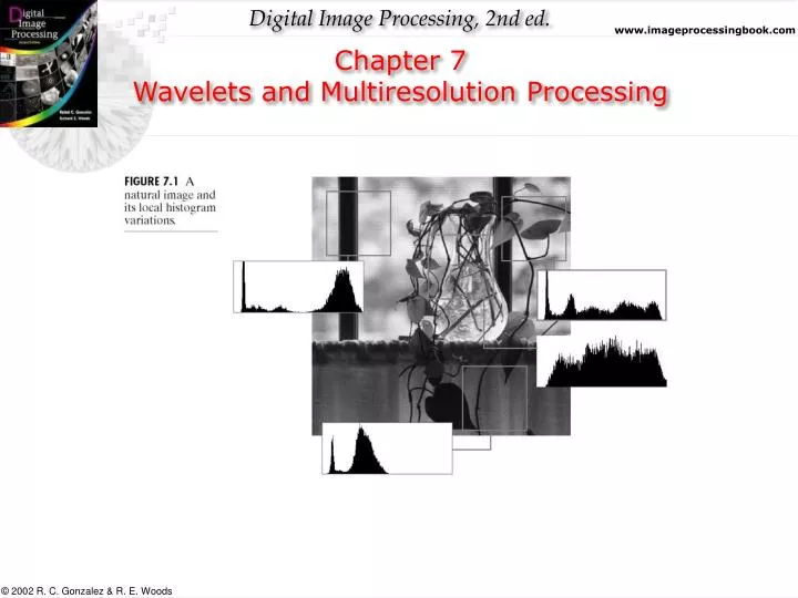
Chapter 7 Wavelets and Multiresolution Processing
Stationary analysis is only applicable to stationary signals. Non-stationary signals require analysis techniques that encompass time variation the short-time Fourier transform wavelets Problem
Speech is stationary within 20ms windows Fourier transforms are calculated for short windows Each transform forms one column of a 3D plot STFT
Each STFT column represents one block of speech Each frequency component has equal bandwidth Each STFT element represents the same time scale and bandwidth as every other component STFT Example
Wavelets allow multi-resolution analysis: That is analysis at different scales or resolution. Standard Fourier analysis only offers a measure of the frequency content of the whole image and the contribution of the image at a particular frequency. Wavelet analysis permits us to describe an image in terms of frequency at a position in the image. Wavelets
Each wavelet component has the same time-bandwidth product Those at low frequencies represent longer periods of time than those at high frequencies A whole variety of wavelets Wavelets
A wavelet decomposition consists of a scaling function and a series of wavelets The scaling function provides the coarse scale The wavelets successively refine the representation Wavelet decomposition
Scaling Function • The four co-efficient scaling function is: and the corresponding wavelet is
Haar Wavelet For example the Haar wavelet is The Wavelet is then
Haar Wavelets • The wavelets are then defined by their coefficients which have to satisfy a set of criteria which are called necessary conditions: For the Haar wavelet c0=c1=1 Length 4 Wavelets must satisfy: When These are Daubechies wavelets
Gabor Wavelet The Gabor wavelet is essentially a sinewave modulated by a Gaussian envelope Where f0 is the modulating frequency, t0 indicates position and a controls the width of the Gaussian envelope. In 2D this becomes, Where x0, y0 control position f0 controls frequency of modulation along either axis and θ controls the direction or orientation of the wavelet.
Examples of 1-D Wavelet Transform From Matlab Wavelet Toolbox Documentation
2-D Example From Usevitch (IEEE Sig.Proc. Mag. 9/01)
Image Pyramids • Creation by iterated approximations and interpolations (predictions) • The approximation output is taken as the input for the next resolution Level • For a number of levels P, two pyramids: approximation (Gaussian) and prediction residual (Laplacian), are created • approximation filters could be: • averaging • low-pass (Gaussian)
Gaussian and Laplacian pyramids Starting image is 512×512; convolution kernel (approximation kernel) is 5×5 Gaussian Different resolutions are appropriate for different image objects (window, vase, flower, etc.) J–3 J–2 J–1 J
Subband Coding • The image is decomposed into a set of band-limited components (subbands). • Two-channel, perfect reconstruction system; two sets of half-band filters • Analysis: h0 – low-pass and h1 – high-pass and Synthesis: g0 – low-pass and g1 – high-pass
Brief reminder of z-transform properties Downsampled and upsampled by a factor of two sequences in z-domain [2↓]x(n)=xdown(n)=x(2n) ⇔Xdown (z)=1[X(z1/2)+X(−z1/2)] 2 [2↑]x(n)=xup(x)=⎧⎨x(n/2) n=0,2,4,... ⇔Xup(z)=X(z2) ⎩ 0 n = 1,3,5,.... Downsampling followed by upsampling x(n)=[2↑][2↓]x(n) ⇔ X(z)=1[X(z)+X(−z)] Z−1(X(−z))=(−1)n x(n)
Chapter 7 Wavelets and Seperable filtering in images
Chapter 7 Wavelets and Multiresolution Processing
Chapter 7 Wavelets and Multiresolution Processing Aliasing is presented in the vertical and horizontal detail subbands. It is due to the down-sampling and will be canceled during the reconstruction stage.
Chapter 7 Wavelets and Multiresolution Processing
Chapter 7 Wavelets and Multiresolution Processing
Chapter 7 Wavelets and Multiresolution Processing
Chapter 7 Wavelets and Multiresolution Processing
Chapter 7 Wavelets and Multiresolution Processing
Chapter 7 Wavelets and Multiresolution Processing
Chapter 7 Wavelets and Multiresolution Processing
•The standard Fourier Transform (FT) decomposes the signal into individual frequency components. •The Fourier basis functions are infinite in extent. •FT can never tell when or where a frequency occurs. •Any abrupt changes in time in the input signal f(t) are spread out over the whole frequency axis in the transform output F(ω) and vice versa. •WT uses short window at high frequencies and long window at low frequencies. It can localize abrupt changes in both time and frequency domains.
Chapter 7 Wavelets and Multiresolution Processing
Chapter 7 Wavelets and Multiresolution Processing
Chapter 7 Wavelets and Multiresolution Processing
Chapter 7 Wavelets and Multiresolution Processing
Chapter 7 Wavelets and Multiresolution Processing
Chapter 7 Wavelets and Multiresolution Processing
Chapter 7 Wavelets and Multiresolution Processing
Chapter 7 Wavelets and Multiresolution Processing
Chapter 7 Wavelets and Multiresolution Processing
Chapter 7 Wavelets and Multiresolution Processing