Download
1 / 15
150 likes | 321 Views
Aggregate Supply & Demand. Introduction & Determinants. Aggregate Demand Curve . (Inverse) Relationship between price level & quantity of aggregate output demanded for the economy as a whole. Aggregate Price Level (measured with GDP deflator).

E N D
Aggregate Supply & Demand Introduction & Determinants
Aggregate Demand Curve • (Inverse) Relationship between price level & quantity of aggregate output demanded for the economy as a whole Aggregate Price Level (measured with GDP deflator) Total quantity of domestic goods & services demanded (= real GDP)
Reasons for Downward Slope • Interest Rate Effect – To get what they want during periods of rising prices, households and firms borrow money or sell assets. This drives up interest rates, reducing investment and consumer spending. • Wealth Effect – A rise in aggregate price level results in a fall in purchasing power and a reduction in consumption. • Net Export Effect – As price levels rise, foreign goods become relatively cheaper and demand for imports rises (while demand for exports falls).
Why the Law of Demand DOESN’T apply • The Law of Demand assumes ceteris paribus, including the assumption that all other goods remain equal – and it is therefore not applicable to the economy as a whole. • Movement up and down the AD curve represents simultaneous change in prices of all final goods and services. This is why the interest rate, wealth, and net export effects provide a better explanation.
Shifts of AD Curve • Changes in AD as a result of price level changes are movements along the curve • Shifts occur when the quantity demanded at a given price level changes – increase to the right, decrease to the left.
Determinants of AD • Shifts occur because of: • Changes in Expectations – future income • Changes in Wealth – value of assets • Size of Existing Stock – incentive for firms • Fiscal Policy – control of demand through government spending and tax policies • Monetary Policy – use of quantity of money and interest rates to stabilize the economy
Short-Run Aggregate Supply Curve Shape of the Curve • Two situations result in SRAS curves with no slope: • Horizontal SRAS curve results from set price level or high unemployment (making wages flexible) • Vertical SRAS curve represents full employment and utilization of resources – so prices can rise, but production cannot.
Short-Run Aggregate Supply Curve • In reality, the curve is normally an upward sloping line as a result of production decisions being based on profitability and the inflexibility of costs in the short-run. • In a perfectly competitive market, when price levels change but costs don’t, the change in profit margin determines quantity produced • In an imperfectly competitive market, producers raise prices and production at times of high demand – and cut prices and production when demand falls
Shifts of SRAS Curve • Changes in aggregate output in response to price level is movement along the curve • Shifts represent changes in the quantity of aggregate output producers are willing to supply at a given aggregate price level – increase to the right, decrease to the left.
Determinants of SRAS • Shifts occur because changes impact per unit cost, like: • Changes in Commodity Prices • Changes in Nominal Wages – Economy-wide • Changes in Productivity
SRAS Scenarios Price Level – Price Level – Price Level – Real GDP – Real GDP – Real GDP –
Long-Run Aggregate Supply Curve • In the long-run, all production costs are flexible. Therefore, in the long run, aggregate price level has no effect on quantity supplied. YP
Potential Output • The horizontal intercept represents an economy’s potential output – the level of production if all prices were fully flexible. • Actual output fluctuates around YP from year to year.
Shifts in LRAS Curve • Growth in potential output over time is the result of rightward shifts of the LRAS curve as a result of: • Increases in quantity of resources • Increases in quality of resources • Improvements in technology
SRAS to LRAS • Economy is always at a point (PL & real GDP) on the SRAS curve. • If that point is not also on the LRAS curve, the SRAS curve will shift until it is. Let’s look at two scenarios…