Download
1 / 47
470 likes | 592 Views
K - + Scattering from D + K - + +. Antimo Palano INFN, Bari R. Andreassen, Brian Meadows University of Cincinnati D. Aston, J. Coleman, W. Dunwoodie, K. Suzuki, D. Leith Group B, SLAC. “Traditional” Dalitz Plot Analysis.

E N D
K-+ Scattering from D+ K-++ Antimo Palano INFN, Bari R. Andreassen, Brian Meadows University of Cincinnati D. Aston, J. Coleman, W. Dunwoodie, K. Suzuki, D. Leith Group B, SLAC
“Traditional” Dalitz Plot Analysis • The “isobar model”, with relativistic Breit-Wigner (RBW) resonant terms, is widely used in studying 3-body decays of heavy quark mesons. • Amplitude for channel {ij}: • Each resonance “R” (mass MR, width R) assumed to have form {12} {23} {13} NR 1 1 1 2 2 2 3 3 3 1 3 2 NR Constant Form factor D form factor spin factor
E791 (WMD) “Model-Independent”Partial-Wave Analysis (MIPWA) • Make partial-wave expansion of decay amplitude in angular momentum of K-+ system produced D form-factor • “Partial Wave:” • Describes invariant mass dependence of K-+ system • -> Related to K-+ • scattering Conserves spin Watson Theorem holds that, up to elastic limit (K’ threshold for S-wave) K phases same as for elastic scattering.
MIPWA (a la WMD / E791) ` • Define S – wave amplitude at discrete points sK=sj. Interpolate elsewhere. model-independent - two parameters(cj, j)per point • P- and D- waves are parametrized by known K* resonances
Unbinned Max. Likelihood Fit • Likelihood function covers 3-dimensions: • s(K1), s(K2) and also the reconstructed 3-body mass MK • Factorize MK dependence: • All events used in signal as well as sidebands have a D+ mass constraint. • Can then overlay Dalitz plot for sideband data directly on signal • Greatly simplifies computation of efficiency. • is efficiency Subscript s is signal Subscript b is background
E791 MIPWA of K-p+S-wave • What does this show ? “It helps reveal a k pole hidden by an Adler zero” - D. Bugg et al.
Compare E791 K-p+S-wave with E791 • Published results are multiplied by the scalar D form-factor used in the analysis. Features similar to previously published k model fit”
Compare E791 K-p+S-wave with LASS • Multiply LASS result by phase space factorMKp / p • Shift LASS phasedownward700 • Good agreement above ~ 1150 MeV/c2 ! • Is there an S-wave D+ (complex) form-factor ?
The BaBar Sample of D+K-++ • Skim carried out byRolf Andreassen. • A likelihood is based on PDFS (signal - MC) and PDFB (background - data sidebands) for each of the following quantities: • SignedD+ decay length l/sl • c2 probability for vertex • PLAB for D+ • Likelihood is product: Skim all with L>2
D+ K-++ Dalitz Plot • Plot includes 500K events (~97% purity) • ~13K are background. • Obviously large S-wave content Interferes with K*(890) (and anything else in P-wave). • Some D-wave also present L > 3 Purity 97%
Three Isobar Model Fits to BaBar Data This is one 2/NDF = 1.3 (NDF=15,600) - very poor fit
E791 S-Wave Fit (on BaBar data) • S-wave is spline with 30 equally spaced points • P-wave is as in model fit, with complex coefficients floated. • D-wave also as in model fit – complex coefficient floated.
K*(1410) K*(1677) K*(1677) K*(1410) • A substantial problem is that we have to assume a form for the P-wave that we know is not correct • It contains no K*(1410) since E791 data did not require this • It is a sum of BW’s – known to violate unitarity (at least). • So, can we find the P-wave the same way ?
Spline Model for P-wave Too • Antimo tried this (see BAD 1291): • Fix P-and D-waves as in the (isobar) model • S(s) from a table of n points. • Now fix S-wave and fit P-wave same way • P(s) from a table of n points. • Fix P-wave and re-fit S-wave • Repeat cycle several times • SIMPLEX • Errors from likelihood scan
|S| S phase S P phase |P| P Antimo’s Result (2 cycles) Im S See BAD 1293 Re S Im P Re P • It is difficult to know if this has converged • or if it is correct
Some MC Tests • Generate 3 toy MC samples, each corresponding to isobar model fits actually made to the BaBar data MCA: S-wave: , K*(1430) P-wave: K*(890), K*(1410), K*(1688) D-wave: K*(1420) MCB: As in MCA, but no D-wave K*(1420) MCC: As in MCA, but no P-wave K*(1410) • Each sample: • No background • ~4M events • Look for self-consistency between fit and generated quantities.
MC Test – S-wave Only Almost perfect fit • S-wave is fitted tospline with 40 equally spaced points • P-wave is fixed as in model fit (but defined as a spline). • D-wave complex coefficient floated. Almost perfect fit Fixed Fixed Almost perfect fit Almost perfect fit OK !
MC Test – P-wave Only • S-wave is fixed as in MCA model fit. • P-wave is fitted tospline with 40 equally spaced points • D-wave complex coefficient floated. Fixed Fixed Almost perfect fit Almost perfect fit Almost perfect fit Almost perfect fit OK !
Migrad (Cycle S- then P-wave) Cycling does work, but convergence seems far away even after 16 cycles! S Goes on forever …? -2lnL P S etc # Function Calls
Mag -2lnL Phase Mag etc # Function Calls MC Test –Magn./Phase Cycles Cycling does work, but convergence seems far away even after 16 cycles! Goes on forever …?
BUT - Float S- and P-waves Together !! Maybe it is not possible tofindboth S- and P-wave amplitudes without a definite form for one of them ??
So – “Read the directions …” • Clearly this is not working! • It also takes far too long as it stands even on 3 GHz CPU: • 8 hours for unbinned fit with1M events and just one wave (30 points) • ~7 days for fit just shown ! Therefore: • Try to understand how this ought to work … • Then improve performance of the fit.
How Does the MIPWA Work? • With structure only in ONE channel (e.g. K-+1) then the density along strips like that shown varies like A + B cos + C cos2 • So we can determine A ~ |S|2 C ~ |P|2 and B ~ |S||P| cos (fs-fP ) i.e., we measure difference|fs-fP| - ambiguous sign Must knoweithersor Pto find the other phase (with ambiguity) S and P only cos
MIPWA for Both S- and P-waves? In this region, below the K*(890) peak, we know P well: So we measure Both S and P over this range Re{P} ? s Im{P}
MIPWA for Both S- and P-waves? Build on this region in horizontalstrips. Measures S and P over this range • [Structure in cross channels: • complicates cos dependence on each strip • but can be measured in this channel. ]
MIPWA for Both S- and P-waves? Bose symmetrize Know S and P everywhere except in the “Gap” Gap
Improve the Fit Performance • Unbinned fit Binned fit • Choose 600x600 bins • Poisson probability Define where is expected number of events in bink observed number of events in bink PDF includes signal & background is normalization (a fit parameter). If bins are small enough, takes care of normalization !!
Improve the Fit Performance • Work with square plot • S(K- +1) vs. cos (K- +2) • Useful features of this kind of fit: • Choosing 600x600 bins (in effect, only about 150K bins) • CPU time independent of actual number of events! • No need to normalize – this is part of the fit. • About 5 times faster for ~ 1 M events.
Improve the Fit Performance • Re- parametrize P-wave: • Spline BWK*1430 x spline • Use Re A & Im A rather than |A| & • More stable where|A| is small • In principal, all fits can now be accomplished in a single step, floating all parameters, in a reasonable time.
Start at “Truth” ~4 M events TRUTH lnL=-16000316.9, chi/NDF146319.2/145889
Different Start ~4 M events Starting model: S-wave: k, K0(1430) P-wave: K*(890), K1*(1677) (No K*1410) D-wave: K2*(1420) lnL=-16000316.9, chi/NDF146314.8/145888
Further Improvement in Fit Performance • Poor performance in 1.0-1.5 GeV/c2 region Due in part to Representation of S-wave near K*(1430) Also results from low statistical content of bins in region • Re- parametrize S-wave: Spline BWK*1430 x spline • Also require at least 10 events in each bin
From 3 Different Starts: ~4 M events lnL=-16000287.4, chi/NDF144250.7/145900
Summary • This kind of fit is shown to work, in principal • By fixing the P-wave up to about 900 MeV/c2 we can now fit S- and P-waves simultaneously. • It seems to add stability if we require bins to have at least 10 events in them. Next: • Add background • Fit data • Systematic / bias studies • Finish BAD
Scattering aReminder Im {T} s h/2 2d T In LASS (s) = 1.0 from threshold up to ~(0.9 –1.0) GeV/c2 x f Re {T} But this may differ in D or B decays Threshold
S S K-p+S- & P-waves from LASS |S| |S| K’ threshold K*(1410) K*(1677) K*(1677) K*(1410)
Partial Waves from Model Fit Phase Magnitude NOTE – no K*(1410) Width of lines represents 1
Omit the “Gap” Region ~4 M events TRUTH lnL=-16000287.1, chi/NDF146240.5/145890
Different Start (and Omit “Gap”) ~4 M events Starting model: S-wave: k, K0(1430) P-wave: K*(890), K1*(1677) (No K*1410) D-wave: K2*(1420) lnL=-16000287.4, chi/NDF146250.7/145900
Watson Theorem • The process P + c can be thought of as Borrowed from M. Pennington (hep-ph/0608016) • The only channel open below elastic limit is elastic scattering, so phase is same as for elastic scattering. • BUT the interaction between c and P introduces overall phase This might also depend on energy, in which case Watson theorem will not apply. FD FR means on mass shell.
Background Model • K-p+p+ invariant mass distribution from sample with L > 3 • Dalitz plot distributions in lower side-band, signal region and upper side-band (log. Scale) • Used directly as input to background function. PDF1b - bin-by-bin interpolation
Second Background • Probable origin • PDF2b = g(MK) x Gauss (M2K) Lost
Efficiency • Efficiency (%) over the Dalitz plot for various laboratory momentum ranges.
Efficiency vs. pLAB • Efficiency (%) vs laboratory momentum. • Lab. momentum for Data (black). • Lab. momentum for reconstructed, signal MC (red). No need to use efficiency as function of pLAB
“Traditional” Model for S-wave - BaBar 2/NDF = 20.1x10³ / 15.6x10³ - a very poor fit
E791 S-Wave Fit (on BaBar data) 2/NDF = 1007/574 – better, but still a poor fit
Add K*(1410) to P-wave - BaBar 2/NDF = 18.8x10³ / 15.5x10³ – Better, but still a very poor fit