Download
1 / 50
500 likes | 531 Views
Markov Random Field. Recap: Graphical Models. Two basic kinds of graphical models Directed graphical models or Bayesian Networks Undirected graphical models or Markov Random Fields Key components Nodes Random variables Edges Directed or undirected

E N D
Recap: Graphical Models • Two basic kinds of graphical models • Directed graphical models or Bayesian Networks • Undirected graphical models or Markov Random Fields • Key components • Nodes • Random variables • Edges • Directed or undirected • The value of a random variable may be known or unknown. Directedgraphical model Undirectedgraphical model unknown known B. Leibe
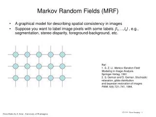
Markov Random Fields • When the probability distribution is strictly positive, it is also referred to as a Gibbs random field, because it can then be represented by a Gibbs measure. • The prototypical Markov random field is the Ising model; indeed, the Markov random field was introduced as the general setting for the Ising model.[1] • In the domain of artificial intelligence, a Markov random field is used to model various low- to mid-level tasks in image processing and computer vision.[2] • For example, MRFs are used for • image restoration, image completion, segmentation, image registration, texture synthesis, super-resolution, stereo matching and Information Retrieval.
Markov Random Field • Markov random field (often abbreviated as MRF), Markov network or undirected graphical model is a set of random variables having a Markov property described by an undirected graph. • A Markov random field is similar to a Bayesian network in its representation of dependencies; the differences being that • Bayesian networks are directed and acyclic, • whereas Markov networks are undirected and may be cyclic. • Thus, a Markov network • can represent certain dependencies that a Bayesian network cannot (such as cyclic dependencies); • on the other hand, it can't represent certain dependencies that a Bayesian network can (such as induced dependencies).
Undirected Graphical Models • Undirected graphical models (“Markov Random Fields”) • Given by undirected graph • Conditional independence is easier to read off for MRFs. • Without arrows, there is only one type of neighbors. • Simpler Markov blanket: B. Leibe Image source: C. Bishop, 2006
Uses of Markov Random Fields • MRFs are a kind of statistical model. • They can be used to model spatial constrains. • smoothness of image regions • spatial regularity of textures in a small region • depth continuity in stereo construction
What are MRFs • Neighbors and cliquesLet S be a set of locations, here for simplicity, assume S a grid.S={ (i, j) | i, j are integers }.Neighbors of sSaredefined as:∂((i, j)) = { (k, l) | 0<(k - i)2 + (l - j)2 <constant }A subset C of S is a clique if any two different elements of C are neighbors. The set of all cliques of S is denoted by Ω.
Examples of neighborhood • 4-neighborhood cliques:
Examples of neighborhood • 8-neighborhood cliques:
Markov Random Fields Node yi: pixel label Edge: constrained pairs Cost to assign a label to each pixel Cost to assign a pair of labels to connected pixels
Markov Random Fields Unary potential 0: -logP(yi = 0 ; data) 1: -logP(yi = 1 ; data) • Example: “label smoothing” grid Pairwise Potential 0 1 0 0 K 1 K 0
Conditional Independence Properties • In an undirected graph, there are three sets of nodes, • denoted A, B, C, and A is conditionally independent • of B given C • Shorthand notation: <=> p(A|B, C) = p(A|C) Conditional independence property
Simple Form • A node will be conditionally independent of all other • nodes conditioned only on neighbouring nodes
Factorization Properties • In a directed graph • Generalized form:
Factorization in MRFs • Factorization • Factorization is more complicated in MRFs than in BNs. • Important concept: maximal cliques • Clique • Subset of the nodes such that there exists a link between all pairs of nodes in the subset. • Maximal clique • The biggest possible such clique in agiven graph. Clique Maximal Clique B. Leibe Image source: C. Bishop, 2006
In an Undirected Graph • Consider two nodes and that are not • connected. • Must be conditionally independent • So, the conditional independence property can be • expressed as The set x of all variables with and removed Factorization Property
Clique • This leads us to consider a graphical concept: • Clique Clique: Maximal Clique:
Potential Function • Define the factors in the potential function by using the clique • Generally, consider the maximal cliques, because other cliques must be the subsets of maximal cliques
Potential Function • Potential function over the maximal cliques of the graph Clique The set of variables in that clique • The joint distribution: Equal to zero or positive • Partition function: a normalization constant
Partition Function • The normalization constant is the major limitations • A model with M discrete nodes each having K states, • then the evaluation involves summing over states • Needed for parameter learning • Exponential growth • Because it will be a function of any parameters that govern the potential functions
Connection between Conditional Independence And Factorization • Define : • For any node , the following conditional property holds • The neighborhood of • All nodes expect • Define : • A distribution can be expressed as • The Hammerley-Clifford theorem states that the sets • and identical.
Potential Function Expression • Restrict the potential function to be positive • It is convenient to express them as exponentials • Energy function • Boltzmann distribution • The total energy is obtained by adding the energies of • each of the maximal energy
Comparison: Directed vs. Undirected Graphs • Directed graphs (Bayesian networks) • Better at expressing causal relationships. • Interpretation of a link: • Conditional probability p(b|a). • Factorization is simple (and result is automatically normalized). • Conditional independence is more complicated. • Undirected graphs (Markov Random Fields) • Better at representing soft constraints between variables. • Interpretation of a link: • “There is some relationship between a and b”. • Factorization is complicated (and result needs normalization). • Conditional independence is simple. B. Leibe
Converting Directed to Undirected Graphs • Simple case: chain We can directly replace the directed links by undirected ones. B. Leibe Slide adapted from Chris Bishop Image source: C. Bishop, 2006
Converting Directed to Undirected Graphs • More difficult case: multiple parents • Need to introduce additional links (“marry the parents”). This process is called moralization. It results in the moral graph. fully connected,no cond. indep.! Need a clique of x1,…,x4 to represent this factor! B. Leibe Slide adapted from Chris Bishop Image source: C. Bishop, 2006
Converting Directed to Undirected Graphs • General procedure to convert directed undirected • Add undirected links to marry the parentsof each node. • Drop the arrows on the original links moral graph. • Find maximal cliques for each node and initialize all clique potentials to 1. • Take each conditional distribution factor of the original directed graph and multiply it into one clique potential. • Restriction • Conditional independence properties are often lost! • Moralization results in additional connections and larger cliques. B. Leibe Slide adapted from Chris Bishop
Example: Graph Conversion • Step 1) Marrying the parents. B. Leibe
Example: Graph Conversion • Step 2) Dropping the arrows. B. Leibe
Example: Graph Conversion • Step 3) Finding maximal cliques for each node. B. Leibe
Example: Graph Conversion • Step 4) Assigning the probabilities to clique potentials. B. Leibe
Comparison of Expressive Power • Both types of graphs have unique configurations. No directed graph can represent these and onlythese independencies. No undirected graph can represent these and onlythese independencies. B. Leibe Slide adapted from Chris Bishop Image source: C. Bishop, 2006