Download
1 / 24
240 likes | 245 Views
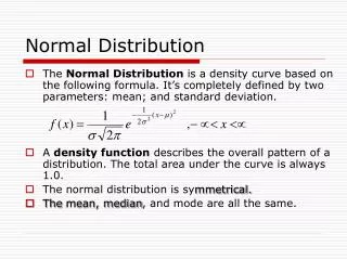
Normal Distribution. Information. Random variables. A random variable , x , is defined as a variable whose values are determined by chance, such as the outcome of rolling a die. A continuous variable is a variable that can assume any values in an interval between any two given values.

E N D
Random variables A random variable, x, is defined as a variable whose values are determined by chance, such as the outcome of rolling a die. A continuous variable is a variable that can assume any values in an interval between any two given values. For example, height is a continuous variable. A person’s height may theoretically be any number greater than zero. What are other example of continuous variables?
Normal distribution The histogram shows the heights of a sample of American women. The histogram is a symmetrical bell-shape. Distributions with this shape are called normal distributions. A curve drawn through the top of the bars approximates a normal curve. height (in) In an ideal normal distribution the ends would continue infinitely in either direction. However, in most real distributions there is an upper and lower limit to the data.
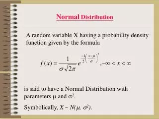
Mean and standard deviation A normal distribution is defined by its mean and variance. These are parameters of the distribution. When the mean is 0 and the standard deviation is 1, this is called the standard normal distribution. the normal distribution:x ~ N(μ, σ2) The random variable, x, has a normal distribution of mean, μ, and variance, σ2.
Continuous distribution The normal distribution is a continuous distribution. In a continuous distribution, the probability that a random variable will assume a particular value is zero. Explain why. For a discrete random variable, as the number of possible outcomes increases, the probability of the random variable being one particular outcome decreases. A continuous variable may take on infinitely many values, so the probability of each particular value is zero. This means that the probability of the random variable falling within a range of values must be calculated, instead of the probability of it being one particular value.
Area under the curve Since all probabilities must fall between 0 and 1 inclusive, the area under the normal distribution curve represents the entire sample space, thus it is equivalent to 100% or 1. The probability that a random variable will lie between any two values in the distribution is equal to the area under the curve between those two values. What is the probability that a random variable will be between μ and positive ∞? The mean divides the data in half. If the area under the curve is 1.00 then the area to one side of the mean is: 1 × 0.5 = 0.5 μ
Applications of normal distributions There are many situations where data follows a normal distribution, such as height and IQ. Some data does not appear to fit the normal curve. However, if many samples are taken from this data, the mean of the samples tends towards a normal distribution. This phenomenon is called the central limit theorem. the central limit theorem: Regardless of the distribution of a population, the distribution of the sample mean will tend towards a normal distribution as the sample size increases.
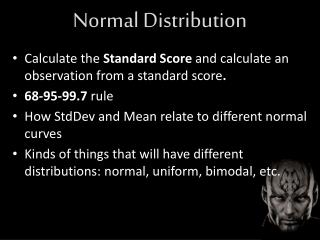
Z-scores Each normally distributed variable has a mean and standard deviation, so the shape and location of these curves vary. All normally distributed variables can be transformed into a standard normally distributed variable using the formula for the standard score, or the z-score. z-score: x – μ z = σ The z-score transforms any normal distribution into a standard normal distribution, with a mean of 0 and a standard deviation of 1.
Standard normal value The z-score tells how many standard deviations any variable is from the mean. If x ~ N(64, 144) represents thescores of an English test, find the z-score for a grade of 49. find the standard deviation: √144 = 12 (x – μ) σ write the z-score formula: z = (49 – 64) 12 substitute in x = 49, μ = 64 and σ = 12: z = solve for the z-score: z = –1.25 The z-score means the grade is 1.25 standard deviations to the left of, or below, the mean.
Standard normal distribution table The area underneath the curve between 0 and the z-score can be found using the standard normal distribution table. The rows show the whole number and tenths place of the z-score and the columns show the hundredths place. Find the area between 0 and a z-score of 0.32. Go down to the “0.3” row. Follow the row across to the “0.02” column. The area between 0 and 0.32 deviations is 0.1255.
Finding values using the z-score If x ~ N(20, 9) represents the amount of time people report spending on electronic devices per week, what values are 2.3 standard deviations away from the mean? state the formula for the z-score: z-score = (x – μ) / σ find the standard deviation: √9 = 3 enter a z-score of –2.3 to find one standard deviation to the left: –2.3 = (x – 20) / 3 x = 13.1 2.3 = (x– 20) / 3 enter a z-score of 2.3 to find one standard deviation to the right: x = 26.9 The values that are one standard deviation from the mean are 13.1 hours and 26.9 hours.
Standard normal distribution table How would you find the area underneath the curve between the z-score and positive infinity? Subtract the area between 0 and the z-score from 0.5 (the area from the mean to infinity). How would you find the area between two z-scores? For z-scores on the same side of the mean, subtract the smaller area from the larger area. For z-scores on the opposite sides of the mean, add the areas.
Practice using Pearson’s Index A 500g bag of flour usually weighs slightly more or less than 500g. The weights of 15 bags are shown. Use Pearson’s Index to decide if the data is skewed. use your graphing calculator to find the mean, median and standard deviation: μ = 500 σ = 2.8 median = 500 substitute into the formula for Pearson’s Index: PI = 3(μ – median) / σ = 3(500 – 500) / 2.8 = 0 analyze: A Pearson’s Index of 0 indicates that the data is not skewed.