Download

1 / 29
290 likes | 296 Views
Flow of mechanically incompressible, but thermally expansible viscous fluids. A. Mikelic, A. Fasano, A. Farina Montecatini, Sept. 9 - 17. LECTURE 1. Basic mathemathical modelling LECTURE 2. Mathematical problem LECTURE 3. Stability.

E N D
Flow of mechanically incompressible, but thermally expansible viscous fluids • A. Mikelic, A. Fasano, A. Farina • Montecatini, Sept. 9 - 17
LECTURE 1. • Basic mathemathical modelling • LECTURE 2. • Mathematical problem • LECTURE 3. • Stability
Viscous fluids, such as molten glass, in many processes aremechanically incompressiblebut experience significant thermal inducedvolume change. In previous lectures we focus on models for viscous fluids that imposethis behavior through a posited internal constraint, followingthe formalism which introduces constraint responsesthat do notproduce entropy. The internal constraint approach yields simpler constitutive relationsand therefore easier material characterization. The internal constraint theory preserves consistency with thethermodynamical balance laws, second lawbutthere is no a prioriguarantee that stability of the rest state is preserved. Indeed the rest state is not stable.
Stability of the rest state means that In this lecture we will analize the stability of the rest state. No energy or momentum sources
Following standard methods (see the original paper by Gibbs [1] • and the recent paper by Bechtel [2]) there are three necessary • and sufficient conditions for stability of the rest state: • Convexity of Gibbs free energy stability • Nonnegativity of Cv • Nonnegativity of the of the so-called bulk modulus [1]. Gibbs, Collected Works, Am. J. Sci. 1878 [2]. Bechtel, Roony, Forest, Int. J. Eng. Sci., 2004
Let us analyze the rest state stability conditions: Condition 3: Nonnegativity of the of the so-called bulk modulus But in the developed theory there is no state equations that link p with the other variables. Such a condition is not clear !
Condition 2: Nonnegativity of Cv But Cv is not defined !! Only Cp is defined. ….so ? ?
Condition 1: Convexity of Gibbs free energy stability Convexity conditions: OK Can be OK NO unless
….. But, may be, y depends also on pressure p !! Answer: y cannot depend on pressure. Indeed, assuming y = y(q, p), the Clausius-Duhem inequality rewrites as Now, this inequality must hold true for all thermo-mechanical processes. Thus, it entails:
Remark According to classical thermodynamics the Gibbs free energy is the Legendre transformationof the Helmoltz free energy, i.e. with But in our case y does not depend on r, and there is no state equation for p. So also condition 1, which appeals to Gibbs free energy, seems not very clear !
Conclusions Although Condition 1 suggests that the rest state is instable, it is not clear if such a method is applicable to our model. Question: How do we proceed ? We try direct analysis
Rest state linear stability Summarizing, once stated the physical assumptions, the mathematical Modeldescribing the dynamics of the fluid is the following1 1 Viscosity m and thermal conductivity K have been considered not depending on temperature
Operating the scaling illustrated in lecture 2, the model can be rewritten as (1) Recall
We may write Non-dimensional characteristic numbers
When the model is used for simulating slow flows of very viscous heated fluids(melted glasses, melted polymer, etc.), often happens that Kr is small and theEckert number is very small (frequently smaller than 10-12). Consequently,the terms containing the Eckert number are dropped in applications and the system reduces to (2) In the sequel we will analyze the linear stability of sistem (1) and (2)
Let us consider the fluid filling all the space and the rest state corresponding to the fluid at rest subject only to a uniform pressureand toisothermal conditions. We now study the linear stability of S,in absence ofany body forces and heat sources.
Let us first linearize the equations considering small (dimensionless) perturbations of the state S, namely In particular, we have2 2As before, for simplifying our analysis we consider Kr constant
We now take the Fourier transform with respect to the spatial variable x of the dependent variable v*, p* andq*. We recall that the Fourier transform, with respect to the spatial variable of a function f (x; t) isdefined by So,
We have to evaluate the eingenvalues of the matrix. Denoting them by li,i = 1; 2; 3 we have Now, since the secular equation is a third degree equation in l¸ whose coefficients are real, at least one eigenvalue is real. The above relations implies thereforethat there exists at least a positive eigenvalue. We thus concludethat the state S is instable.
We now consider the linear stability of system (2).Proceeding as before
W In particular, and so Concerning p, we have p 0 as t
We therefore conclude that, if the dynamics is governed by system (2), then the state S is linearly stable.
Proposed remedies • Bechtel and coworkers proposed the constraint r=r(s). Actually • such a constraint was studied by Scott [3] in the context • of linear thermoelasticity. • Rajagopal [4] and coworkers propose to first develop the constitutive • theories for unconstrained materials, eliminating, if necessary, • pathological behavior by suitable restrictions on the functions • (convexity, positivity definiteness, etc. ) and then obtaining the • constrained for by a carefully chosen limiting process [3] Scott 1992, Q.J. Mech. Appl. Math. [4] Rajagopal et Al., Proc. R. Soc. Lond. (2004)