Download
1 / 68
730 likes | 1.04k Views
Motion Segmentation. By Hadas Shahar (and John Y.A.Wang , and Edward H. Adelson , and Wikipedia and YouTube). Introduction. When given a video input, we would like to divide it into segments according to the different movement types. This is useful for object tracking and

E N D
Motion Segmentation By HadasShahar (and John Y.A.Wang, and Edward H. Adelson, and Wikipedia and YouTube)
Introduction • When given a video input, we would like to divide it into segments according to the different movement types. • This is useful for object tracking and video analysis
Session Map • Building Blocks: • Layered Image representation • Optic Flow Estimation • Affine Motion Estimation • Algorithm Walkthrough • Examples
Session Map • Building Blocks: • Layered Image representation • Optic Flow Estimation • Affine Motion Estimation • Algorithm Walkthrough • Examples
Layered Image Representation • Given a simple movement, what would be the best way to represent it? • Which parameters would you select to represent for the following scene?
Layered Image Representation For any movement we would like to have 3 maps: • The Intensity Map • The Alpha Channel (or- opacity) • The Warp Map (or- optic flow)
For example, if we take a scene of a hand moving over a background, we would like to get:
Given these maps, it’s possible to easily reproduce the occurring movement. • But how can we produce these maps?
Session Map • Building Blocks: • Layered Image representation • Optic Flow Estimation • Affine Motion Estimation • Algorithm Walkthrough • Examples
Optic Flow Estimation(this is the heavy part) • The Optical Flow is a field of vectors describing the movement in the image • For example:
Optic Flow Estimation(this is the heavy part) • Note! Optical Flow doesn’t describe the occurring movement, but the movement we perceive. Look at the Barber’s pole for example
Optic Flow Estimation(this is the heavy part) • The actual motion is RIGHT • But the perceived motion (or- Optical Flow) is UP
Optic Flow Estimation- the Lucas-Kanade method In order to identify movements correctly, we have to work with several assumptions: • Brightness Consistency- the movement won’t affect the brightness of the object • Constant Motion in a neighborhood- neighboring pixels will move together
Optic Flow Estimation- the Lucas-Kanade method Definitions: X(t) is the point X at time t (X=x,y) I(X(t)) is the brightness of point X at time t. is the gradient.
Optic Flow Estimation- the Lucas-Kanade method Brightness Consistency Assumption: I(x(t),t)= constfor any t Meaning- the brightness of point x(t) is constant. Therefore the time derivative must be 0: We would like to focus on this part, the velocity
Optic Flow Estimation- the Lucas-Kanade method But why is the Intensity assumption not enough? Let’s look at the following example and try to determine the optical flow:
Optic Flow Estimation- the Lucas-Kanade method It looks like the grid is moving down and to the right But it can actually be one of the following:
Optic Flow Estimation- the Lucas-Kanade method Since our window of observation is too small, we can’t infer the actual motion taking place. This is called the Aperture Problem And this is why we need the 2nd constraint
Optic Flow Estimation- the Lucas-Kanade method Constant Motion In a Neighborhood: We assume the velocity is the same in our entire window of observation- W(x) is the window or- environment, of x
Optic Flow Estimation- the Lucas-Kanade method There is a trade off here- The larger the window the less accurately it represents the velocity (since we assume the velocity is constant there) And in the other direction- the smaller the window the more likely we are to have the aperture problem
Optic Flow Estimation- the Lucas-Kanade method Sadly, since there are some changes in intensity (due to environment changes or even sensor noise) –the derivative will never actually be 0. So, we take the least square error:
Optic Flow Estimation- the Lucas-Kanade method The minimal value will occur when the 2nd derivative is 0: When: So V is:
Optic Flow Estimation- the Lucas-Kanade method A few notes regarding M: M is a 2x2 matrix -made up of the gradient times its transpose: We can divide M into 3 cases (this is going to be very similar to the Harris corner detection)
Optic Flow Estimation- the Lucas-Kanade method Case1: If the gradient is 0, M=0,there are no eigenvalues and V can have any value. This occurs when our window is at a clear region:
Optic Flow Estimation- the Lucas-Kanade method Case2: If the gradient is constant, M is not 0 but we’ll receive only 1 eigenvalue. This occurs when our window is at an edge:
Optic Flow Estimation- the Lucas-Kanade method Case1: If M is invertible (det=0), we can find Veasily This occurs when our window is at a corner:
Optic Flow Estimation- the Lucas-Kanade method After we find V for every window, we get Velocity vector map, or- the Optical Flow.
Session Map • Building Blocks: • Layered Image representation • Optic Flow Estimation • Affine Motion Estimation • Algorithm Walkthrough • Examples
Affine Estimation • In Affine Estimation, we assume our motions can be described by affine transformations. • This includes: • Translations • Rotations • Zoom • Shear And this does cover a lot of the motions we encounter in the real world
Affine Estimation The idea behind Affine Estimation is quite simple- Find the affine transformation between 2 images, that will have the minimal difference.
Affine Estimation Quick reminder:
Affine Estimation There are several ways to do this, most commonly by matching feature-points between the 2 images and calculating the Affine transformation matrix (remember?) What we’ll use won’t be based on feature points, but on the Velocity vector calculated from the Optical Flow. We’ll get to that later though, so for now- no formulas!
Session Map • Building Blocks: • Layered Image representation • Optic Flow Estimation • Affine Motion Estimation • Algorithm Walkthrough • Examples
Part 2- The Algorithm Walkthrough • So how can we combine all the information we gathered so far into creating our 3 maps for every frame?
The Algorithm Walkthrough • Here’s the basic idea:
The Algorithm Walkthrough • Here’s the basic idea: First, we calculate the Optical Flow- this gives us the Warp map. But since it will only look for 1 overall motion, it may disregard object boundaries and we’ll get several different objects in our motion.
The Algorithm Walkthrough • Here’s the basic idea: Then, we divide the image(s) into arbitrary sub-regions, and use Affine Estimation, which helps us find the local motions within every sub-region
The Algorithm Walkthrough • Here’s the basic idea: Then we check the difference between our initial guess and the movement observed. And reassign the sub-regions to minimize the error
Hypothesis Testing Our estimation using an affine transformation Actual change
The Algorithm Walkthrough • Here’s the basic idea: We repeat the cycle iteratively, constantly refining the motion estimation. Convergence is achieved when either: Only a few points are reassigned in each iteration Max number of iterations is reached
Region reassignments- in each iteration we refine our estimation results This segmentation is what provides us with the Opacity Map
The Algorithm Walkthrough Reminder- This is an Affine Transformation matrix: Made up of 6 variables, to cover the rotation, translation, zoom and shear operations
The Algorithm Walkthrough- definitions Let V be our Velocity (obtained by the Optical Flow estimation) We would like to use the velocity to represent the Affine Transformation: But how can we work with V in such a way? We break V into Vx and Vy, 2 vectors representing the velocity in the X and Y direction respectively
The Algorithm Walkthrough- definitions Vx(x,y)= [aX, bY, c] Vy(x,y)= [dX, eY, f] Where a,b,c,d,e,f are the variables of the affine transformation
The Algorithm Walkthrough- definitions • Let be the ith hypothesis vector. Meaning- is the affine transformation matrix we believe would best represent the ith region’s movement. • We would like to break H into its x and y parts as well:
The Algorithm Walkthrough- definitions And last but not least- We define *That’s our original coordinates vector