Download
1 / 41
410 likes | 422 Views
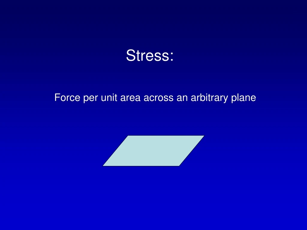
Stress:. Force per unit area across an arbitrary plane. Stress Defined as a Vector. ^. ^. N = unit vector normal to plane t(n) = (t x ,t y ,t z ) = traction vector. The part of t that is perpendicular to the plane is normal stress

E N D
Stress: Force per unit area across an arbitrary plane
Stress Defined as a Vector ^ ^ N = unit vector normal to plane t(n) = (tx,ty,tz) = traction vector The part of t that is perpendicular to the plane is normal stress The part of t that is parallel to the plane is shear stress
Stress Defined as a Tensor z ^ txz y x z tzx ^ t(y) t(z) x t(x) ^ No net rotation • txxtxytxz t = t T =tyxtyytyz tzxtzytzz
Relation Between the Traction Vector and the Stress Tensor z ^ txz y x z tzx ^ t(y) t(z) x t(x) ^ No net rotation ^ • tx(n) txxtxytxz nx t(n) = t n=ty(n) = tyxtyytyz ny tz(n) tzxtzytzz nz ^ ^ ^ ^ ^ ^ ^
Relation Between the Traction Vector and the Stress Tensor That is, the stress tensor is the linear operator that produces the traction vector from the normal unit vector…. ^ • tx(n) txxtxytxz nx t(n) = t n=ty(n) =tyxtyytyz ny tz(n) tzxtzytzz nz ^ ^ ^ ^ ^ ^ ^
Principal Stresses • Most surfaces has both normal and tangential (shear) traction components. • However, some surfaces are oriented so that the shear traction = 0. • These surfaces are characterized by their normal vector, called principal stress axes • The normal stress on these surfaces are called principal stresses • Principal stresses are important for source mechanisms
Stresses in a Fluid If t1=t2=t3, the stress field is hydrostatic, and no shear stress exists • -P 00 • t = 0-P 0 00-P P is the pressure
Pressure inside the Earth Stress has units of force per area: 1 pascal (Pa) = 1 N/m^2 1 bar = 10^5 Pa 1 kbar = 10^8 Pa = 100 MPa 1 Mbar = 10^11 Pa = 100 GPa Hydrostatic pressures in the Earth are on the order of GPa Shear stresses in the crust are on the order of 10-100 MPa
Pressure inside the Earth At depths > a few km, lithostatic stress is assumed, meaning that the normal stresses are equal to minus the pressure (since pressure causes compression) of the overlying material and the deviatoric stresses are 0. The weight of the overlying material can be estimated as rgz, where r is the density, g is the acceleration of gravity, and z is the height of the overlying material. For example, the pressure at a depth of 3 km beneath of rock with average density of 3,000 kg/m^3 is P = 3,000 x 9.8 x 3,000 ~ 8.82 10^7 Pa ~ 100 MPa ~ 0.9 kbar
Mean (M) and Deviatoric (D) Stress • txxtxytxz t =tyxtyytyz tzxtzytzz M = txx + tyy + tzz = tii/3 • txx-M txytxz D=tyxtyy-M tyz tzxtzytzz-M
Strain: Measure of relative changes in position (as opposed to absolute changes measured by the displacement) U(ro)=r-ro E.g., 1% extensional strain of a 100m long string Creates displacements of 0-1 m along string
J can be divided up into strain (e) and rotation (Ω) is the strain tensor (eij=eji) ux ux uy ux uz x y x z x ½( + ) ½( + ) e = uy ux uy uy uz x y y z y ½( + ) ½( + ) uz ux uz uy uz x z y z z ½( + ) ½( + )
J can be divided up into strain (e) and rotation (Ω) ux uy ux uz y x z x 0 ½( - ) ½( - ) Ω= uy ux uy uz x y z y -½( - ) 0 ½( - ) uz ux uz uy x z y z -½( - ) -½( - ) 0 is the rotation tensor (Ωij=-Ωji)
Volume change (dilatation) • = 1/3 ( + + ) = tr(e) = div(u) • > 0 means volume increase • < 0 means volume decrease ux uy uz x y z ux x ux x >0 <0
∂2ui/∂t2 = ∂jij + fi= Equation of motion= Homogeneous eom when fi=0
Seismic Wave Equation (one version) For (discrete) homogeneous media and ray theoretical methods, we have ∂2ui/∂t2= ()·u-xxu
Plane Waves: Wave propagates in a single direction u(x,t) = f(tx/c) travelling along x axis = A()exp[-i (t-s•x)] = A()exp[-i(t-k•x)] where k= s = (/c)s is the wave number ^
s x sin = vt, t/x = sin/v = u sin = p u = slowness, p = ray parameter (apparent/horizontal slowness) rays are perpendicular to wavefronts x s wavefront at t+t wavefront at t
p = u1 sin 1 = u2 sin 2 u = slowness, p = ray parameter (apparent/horizontal slowness) 1 v1 2 v2
p = u1sin 1= u2sin 2= u3sin 3 Fermat’s principle: travel time between 2 points is stationary (almost always minimum) 1 v1 2 v2 3 v3
Continuous Velocity Gradients p = u0sin 0= usin = constant along a single ray path X v z 0 =90o,u=utp T dT/dX = p = ray parameter X
X(p) generally increases as p decreases -> dX/dp < 0 X v z p decreasing =90o,u=utp T Prograde traveltime curve X
X(p) generally increases as p decreases but not always X v z Prograde Retrograde T caustics Prograde X
Reduced Velocity Prograde Retrograde T caustics Prograde X T-X/Vr X
X(p) generally increases as p decreases -> dX/dp < 0 Shadow zone X v z lvz T X p
j Traveltime tomography T = ∫ 1/v(s)ds = ∫u(s)ds Tj = ∑ Gij ui Tj = ∑ Gijui i=1 d=Gm GTd=GTGm mg=(GTG)-1GTd j-th ray i=1
Earthquake location uncertainty n i=1 2 = ∑ [ti-tip]2/i2 i expected standard deviation 2 (mbest)= ∑ [ti-tip(mbest)]2/ndf mbest is best-fitting station 2(m) = ∑ [ti-tip]2/2 - contour! n i=1 n i=1
Fast location: S-P times: D ~ 8 x S-P(s)
Other sources of error: Lateral velocity variations slow fast Station distribution
Emean = 1/2 A2 2 (higher frequencies carry more E!) A2/A1= (1c1/2c2)1/2 ds2 ds1
1cos1-2cos2 S’S’’= 1cos1+2cos2 2 1cos1 S’S’ = 1cos1+2cos2 since ucoscos For vertical incidence ( 1 -2 A1’’= 1 +2 2 1 A2’ = 1 +2 1-2 2 1 S’S’’vert= S’S’vert= 1+2 1+2
S waves vertical incidence P waves vertical incidence: 1-2 2 1 P’P’’vert= - P’P’vert= 1+2 1+2 1-2 2 1 S’S’’vert= S’S’vert= 1+2 1+2
E1flux = 1/2 c1A12 2 cos1 E2flux = 1/2 c2A22 2 cos2 Anorm = [E2flux/E1flux]1/2 = A2/A1 [c2cos2/c1cos1]1/2 = Araw [c2cos2/c1cos1]1/2 1cos1-2cos2 S’S’’norm= = S’S’’raw 1cos+2cos 2 1cos (c2cos2)1/2 S’S’norm = x 1cos1+2cos2 (c1cos1)1/2
2 1cos S’S’ = 1cos+2cos What happens beyond c ? There is no transmitted wave, and cos = (1-p2c2)1/2 becomes imaginary. No energy is transmitted to the underlying layer, we have total internal reflection. The vertical slowness =(u2-p2)1/2 becomes imaginary as well. Waves with Imaginary vertical slowness are called inhomogeneous or evanescent waves.
Phase changes: Vertical incidence, free surface: S waves - no change in polarity P waves - polarity change of Vertical incidence, impedance increases: S waves - opposite polarity P waves - no change in polarity Fig 6.4 Phase advance of /2 - Hilbert Transform
Attenuation: scattering and intrinsic attenuation Scattering: amplitudes reduced by scattering off small-scale objects, integrated energy remains constant Intrinsic: 1/Q() = -E/2E E is the peak strain energy, -e is energy loss per cycle Q is the Quality factor A(x)=A0exp(-x/2cQ) X is distance along propagation distance C is velocity
Ray methods: t* = ∫dt/Q ( r ), A()=A0()exp(-t*/2) i.e., higher frequencies are attenuated more! pulse broadening