Download
1 / 38
380 likes | 391 Views
Chapter 03 Decrease-and-Conquer. Decrease-and-Conquer Exploiting the relationship between a solution to a given instance of a problem and a solution to a smaller instance of the same problem. Once such a relationship is established, the decrease-and-conquer technique can be exploited

E N D
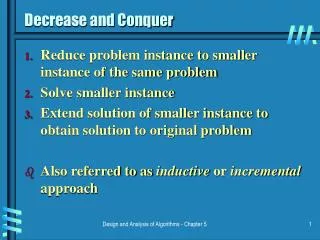
Decrease-and-Conquer • Exploiting the relationship between • a solution to a given instance of a problem and • a solution to a smaller instance of the same problem. • Once such a relationship is established, the decrease-and-conquer technique can be exploited • either top down (- a recursive implementation, and may be non-recursive) • or bottom up (- iterative implementation, also called incremental approach).
There are three major variations of decrease-and-conquer: • Decrease by a constant • Strategy: Reduce the size of an instance by the same constant on each iteration of the algorithm. • Decrease by a constant factor • Strategy: Reduce a problem’s instance by the same constant factor on each iteration of the algorithm. • Variable size decrease • Strategy: A size reduction pattern varies from one iteration of an algorithm to another.
An example of decrease-by-one: • Consider the exponentiation problem of computing an,where a ≠0 • and n is positive integer 1, 2, 3, …. (or n is a nonnegative integer). • The relationship between a solution to an instance of size n and an instance of size n-1 is obtained by the formula: an = an-1 * a. • So the function f(n) = an can be computed: • either “top-down” by using its recursive definition
Decrease by a constant • either “top-down” by using its recursive definition • f(n-1)* a if n > 1 • f(n) = • a if n = 1 (or 1 if n =0) …(3.1) • or “bottom up” by multiplying a by itself n-1 times (or 1 by a n times). (This is the same as the brute-force algorithm). (iterative) • an = a * a * … * a or 1 * a * a * … * a • n-1 times * n times *
Decrease-by-one Example 3.1: Compute the factorial function F(n) = n! based on the factorial n! definition: n! = 1 * 2 * … * (n-1) * n for any nonnegative integer n ≥ 1, and 0! = 1 Then we can compute F(n) = F(n-1) * n with the following recursive algorithm. Algorithm F(n) //Compute n! recursively //Input: A nonnegative integer n //Output: The value of n! if n = 0 return 1 else return F(n-1) * n Top-down approach
Decrease by a constant • Consider the top-down approach (3.1): • Let M(n) be the number of multiplication operations needed. • M(n) = M(n -1) +1 when n >1 • M(1) = 0 • Solution • M(n) = M(n-2) +1 + 1, where M(n-1) = M(n-2) + 1. • M(n) = M(n – i) + i • Let i = n-1. Then M(n) = M(n – (n-1)) + n-1 • = M(1) + n – 1 • = 0 + n – 1 • = n -1 = ϴ(n)
The decrease-by-a-constant-factor technique • Strategy: Reduce a problem’s instance by the same constant factor on each iteration of the algorithm. • Decrease-by-a-constant-factor algorithms usually run in logarithmic time. • An example • The Binary Search is an example of decrease-by-half. • The worst-case time efficiency of binary search, T(n) = ϴ(log2 n).
An example of decrease-by-half: • For the exponentiation problem, if the instance of size n (for an even n only) is to compute an, the instance of half its size will be to compute an/2 [decrease-by-half], with the relationship between the two: an = (an/2)2. • If n is odd, we have to compute an-1, by using the rule for even-valued exponents and then multiply the result by a. • (an/2)2 if n is even and positive • an = (a(n-1)/2)2 * a if n is odd • 1 if n = 0. (3.2) A brute force approach: Reducing by a constant (using top-down approach, a recursive call, (3.1) ) takes ϴ(n).
If we compute anrecursively according to formula (3.2), • we measure the algorithm’s efficiency by the number of multiplications, • and the algorithm to be in O(log n). • The reason is that, on each iteration, the size is reduced by at least one half at the expense of no more than two multiplications [if n is odd.].
M(n) = M(n/2) + 1 where n > 1 M(1) = 0 Solution: Let n =1, an = a. Let n = . n = implies that k = log n M(n) = M( ) = M( ) + 1 = M() + i = M() + k by setting i = k = M(1) + k = k = log n Pbm: Cut any stick into an unit stick. n 63 1 n
Based on the divide-and-conquer • Note a difference between this algorithm and the one based on the divide-and-conquer idea of solving two instances of the exponentiation problem of size n/2: • a└n/2┘* a┌n/2┐ if n > 1 • an = • a if n = 1 (2.3) • The algorithm based on formula (2.3) is inefficient (why?), whereas the one based on (3.2) if much faster. • M(n) = M(└n/2┘) + M(┌n/2┐ ) + 1 • M(1) = 0 (2.3) Pbm: Cut any stick into an unit stick.
Based on the divide-and-conquer The recurrence relation for computing efficiency based on the number of multiplications: M(n) = M(└n/2┘) + M(┌n/2┐) + 1 if n > 1 M(1) = 0 if n = 0 Let n = . Solve the recurrence relation for the number of multiplications based on divide-and-conquer, using Master Theorem: Θ( nd ) = f(n) = 1. That is, d = 0 Since a = 2 and b = 2, and bd = 1, then a > bd . That is, M(n) = Θ( ), where logba = log22 = Θ( n)
Or, M(n) = 2 M(n/2) + 1 and M(1) = 0 Let n = 2k .M(n) = 2M(2k-1 ) + 1 = 2(2M(2k-2 ) + 1) + 1 = 22 M(2k-2 ) + 2 + 1 = 23 M(2k-3 ) + 22 + 2 + 1 = 2i M(2k-i ) + 2i-1 + … + 22 + 2 + 1 = 2k M(2k-k ) + 2k-1 + … + 22 + 2 + 1 = 0 + 2k-1 + … + 22 + 2 + 1 = 2k – 1= n – 1 = Θ( n)
The variable-size-decrease technique • Strategy: A size reduction pattern varies from one iteration of an algorithm to another. • Euclid’s algorithm for computing the greatest common divisor is a good example.
The variable-size-decrease technique • Recall that this algorithm is based on the formula • gcd(m, n) = gcd(n, m mod n) • for any nonnegative integer m {i.e., 0, 1, …} and any positive integer n < 0. • Then, • Algorithm Euclid(m, n) • // input: m and n are arbitrary nonnegative integers • if n = 0 then return m • else return Euclid(n, m mod n);
The running time of Euclid’s algorithm Analyze the worse-case running time of Euclid as a function of the size of m and n. Assume that m > n ≥ 0. If m < n, Euclid spends one recursive call swapping its arguments m and n, and then proceeds. The overall running time of Euclid is proportional to the number of recursive calls it makes. Our analysis makes use of the Fibonacci number Fk. Lemma 0.1 If m > n ≥ 1 and the invocation Euclid(m, n) performs k ≥ 1 recursive calls, then m ≥ Fk+2 and n ≥ Fk+1. Theorem 0.5 (Lame’s Theorem) For any integer k ≥ 1, if m > n ≥ 1 and n < Fk+1, then the call Euclid(m, n) makes fewer than k recursive calls.
The running time of Euclid’s algorithm Since Fk is approximately k/√5, where is the golden ratio , the number of recursive calls is O(log n). For the worst case number of recursive calls for the Euclid algorithm is O(s t). wheres = └ log m ┘ + 1 bits and t = └ log n ┘ + 1 bits. The run time complexity is O((log m)(log n) bit operations. It follows that if Euclid is applied to two ß-bit numbers, then it will perform O(ß) arithmetic operation and O(ß3 ) bit operations (assuming that multiplication and division of ß-bit numbers take O(ß2 ) bit operations).
Common Recurrence Types in Algorithm Analysis Decrease-by-one A decrease-by-one algorithm solves a problem by exploiting a relationship between a given instance of size n and a smaller instance of size n-1. Specific examples include recursive evaluation of n! and Insertion sort:
Decrease-by-one Example 3.1: Compute the factorial function F(n) = n! based on the factorial n! definition: n! = 1 * 2 * … * (n-1) * n for any nonnegative integer n ≥ 1, and 0! = 1 Then we can compute F(n) = F(n-1) * n with the following recursive algorithm. Algorithm F(n) //Compute n! recursively //Input: A nonnegative integer n //Output: The value of n! if n = 0 return 1 else return F(n-1) * n Top-down approach Time efficiency is ϴ(n)
Example 3.2: Insertion sort: Using iteration of insertion sort, A[i] is inserted in its proper position among the preceding elements previously sorted. A[0] ≤ A[1] ≤ A[2] ≤ … A[j] < A[j+1] ≤ … ≤ A[i-1] | A[i] … A[n-1] Smaller than or equal to A[i] greater than A[i]
Algorithm InsertionSort(A[0..n-1]) //Sorts a given array by insertion sort. //Input: An array A[0..n-1] of an orderable elements. //Output: Array A[0..n-1] sorted in nondecreasing order. for i ← 1 to n-1 do { v ← A[i]; j ← i -1; while j ≥ 0 and A[j] > v do { A[j+1] ← A[j]; //move the elements of A[j] to the //right into A[j+1]; open a slot for v j ← j – 1; } //end while-do A[j+1] ← v; }//end for-do
Analysis of algorithm • The basic operation of the algorithm is the key comparison A[j] > v not j ≥ 0 (why)? j ≥ 0 is a sentinel (we need this to halt the algorithm if for all j, A[j] > A[i] ). • The number of key comparisons in this algorithm obviously depends on nature of the input. {Then we have worst-, best- and average-cases}
In the worst case, • A[j] > v is executed the largest number of times, i.e., for every j = i – 1, 2, … , 0. Since v = A[i], it happens if and only if A[j] > A[i] for j = i – 1, 2, …, 0. • Thus for the worst-case input, we get A[0] > A[1] (fori = 1 ), A[1] > A[2] (fori = 2) , … , A[n-2] > A[n-1] (fori = n-1 ). • In other words, the worst case input is an array of strictly decreasing values. The number of key comparisons for such an input is • for i ← 1 to n-1 do { • … • while j ≥ 0 and A[j] > v do { • … } //end while-do • … }//end for-do • Cworst(n) = = ε Θ(n2 ).
In the best case, • the comparison A[j] > v is executed only once on every iteration of the outer loop. • It happens if and only if A[i-1] ≤ A[i] for everyi = 1, …., n-1, i.e., if the input array is already sorted in ascending order. • Thus, for sorted arrays, the number of key comparisons is • Cbest(n) = = (n-1) ε Θ(n). • The very good performance in the best case of sorted arrays is not very useful by itself, because we cannot expect such convenient inputs.
In the average-case, • A rigorous analysis of the algorithm’s average-case efficiency is based on investigating the number of element pairs that are out of order. • It shows that on randomly ordered arrays, insertion sort makes on average half as many comparisons as on decreasing arrays, i.e., • Cavg(n) ≈ ε Θ(n2 ). { • = • ≈ }
The recurrence equation for investigating the time efficiency of such algorithms typically has the form T(n) = T(n - 1) + f(n) (3.4) where function f(n) accounts for the time needed to reduce an instance to a smaller one and to extend the solution of the smaller instance to a solution of the larger instance. Reduce by one algorithms
Applying backward substitution to (3.4) yields T(n) = T(n-1) + f(n) = [T(n-2) + f(n-1)] + f(n) = … = T(n-i) + f(n –i+1) + … + f(n-2) + f(n-1) + f(n) = T(0) + f(1) + f(2) + … + f(n-2) + f(n-1) + f(n) = T(0) +
Now, we have T(n) = T(0) + . For a specific function f(x), the sum can be either computed exactly or its order of growth ascertained. For example, if f(n) = 1, = n; if f(n) = log n, ε Ɵ(nlog n); if f(n) = nk , ε Ɵ(nk+1 )
Decreased-by-a-constant-factor A decrease-by-a-constant-factor algorithm solves a problem by reducing its instance of size n to an instance of size n/b (b = 2 for most but not all such algorithms), solving the smaller instance recursively, and then, if necessary,extending the solution of the smaller instance to a solution of the given instance. The most important example is binary search: Compare a search key K with the array’s middle element A[m]. If they match, the algorithm stops; otherwise, the same operation is repeated recursively for the first half of the array if K < A[m], and for the second half if K > A[m]:
Algorithm BinarySearch(A[0 .. n-1], K) //Implements nonrecursive binary search //Input: An array A[0 .. n-1] sorted in ascending order and // a search key K //Output: An index of the array’s element that is equal to K // or -1 if there is no such element p ← 0; r ← n - 1; while p ≤ r do m ← └ (p + r) /2 ┘; if K = A[m] return m else if K < A[m] then r ← m - 1 else p ← m + 1; //end if-else-if-else return -1; //end while-do
Other examples for the Decreased-by-a-constant-factor include: • Compute anrecursively by using the exponentiation by squaring. • The multiplication a la russe(also called Russian peasant method). • Let n and m be positive integers. Compute the product of n and m using: • if n is even • n * m = • if n is odd • And the fake-coin problem, and the Josephus Problem.
The recurrence equation for investigating the time efficiency of such decrease-by-a-constant-factor algorithms typically has the form T(n) = T(n/b) + f(n) (3.5) where b > 1 and function f(n) accounts for the time needed to reduce an instance to a smaller one and to extend the solution of the smaller instance to a solution of the larger instance. Strictly speaking, equation (3.5) is valid only for n = bk,k = 0, 1, …For values of n that are not the powers of b, there is typically some round-off, usually involving the floor and/or ceiling functions. The standard approach to such equations is to solve them for n = bkfirst. Afterward, either the solution is tweaked to make it valid for all n’s,or the order of growth of the solution is established based on the smoothness rule (Theorem 2.2).
T(n) = T(n/b) + f(n) By considering n = bk , k = 0, 1, 2, …. and applying backward substitutions to (B.13), we have T(n) = T(bk ) = T(bk-1 ) + f(bk ) = T(bk-2 ) + f(bk-1 )+ f(bk ) = … = T(bk-i ) + f(bk-i+1 ) + … + f(bk-2 ) + f(bk-1 )+ f(bk ) = T(1) + leti = k
So far, we have T(n) = T(bk ) = T(1) + For a specific function f(x),the sum can be eithercomputed exactly or its order of growth ascertained. For example, if f(n) = 1, = k = logb n. If f(n) = n, = = b( ) = b ( )
Note that recurrence T(n) = T(n/b) + f(n) (3.5) is a special case of recurrence for Divide-and-conquer T(n) = aT(n/b) + f(n) which is covered by the Master Theorem (Theorem 2.3). According to this theorem, in particular, if f(n) ε Ω( nd ) where d > 0, then T(n) ε Ω( nd ) as well.
Decomposition of Graph • In the remaining of this chapter, we will cover graphs, • including Depth-First Search and Breadth-First Search • and Topological Sorting