Download
1 / 84
840 likes | 858 Views
FK6163. T Test, ANOVA & Proportionate Test. Assoc. Prof . Dr Azmi Mohd Tamil Dept of Community Health Universiti Kebangsaan Malaysia. T-Test. Independent T-Test Student’s T-Test Paired T-Test ANOVA. Student’s T-test.

E N D
FK6163 T Test, ANOVA & Proportionate Test Assoc. Prof . Dr Azmi Mohd TamilDept of Community HealthUniversiti Kebangsaan Malaysia
T-Test Independent T-Test Student’s T-Test Paired T-Test ANOVA
Student’s T-test William Sealy Gosset @ “Student”, 1908. The Probable Error of Mean. Biometrika.
Student’s T-Test • To compare the means of two independent groups. For example; comparing the mean Hb between cases and controls. 2 variables are involved here, one quantitative (i.e. Hb) and the other a dichotomous qualitative variable (i.e. case/control). • t =
Examples: Student’s t-test • Comparing the level of blood cholestrol (mg/dL) between the hypertensive and normotensive. • Comparing the HAMD score of two groups of psychiatric patients treated with two different types of drugs (i.e. Fluoxetine & Sertraline
Assumptions of T test • Observations are normally distributed in each population. (Explore) • The population variances are equal. (Levene’s Test) • The 2 groups are independent of each other. (Design of study)
Sample size > 30 Small sample size, equal variance Manual Calculation
Hypertensive :Mean : 214.92s.d. : 39.22 n : 64 Normal :Mean : 182.19s.d. : 37.26 n : 36 Example – compare cholesterol level • Comparing the cholesterol level between hypertensive and normal patients. • The difference is (214.92 – 182.19) = 32.73 mg%. • H0 : There is no difference of cholesterol level between hypertensive and normal patients. • n > 30, (64+36=100), therefore use the first formula.
Calculation • t = (214.92- 182.19)________ ((39.222/64)+(37.262/36))0.5 • t = 4.137 • df = n1+n2-2 = 64+36-2 = 98 • Refer to t table; with t = 4.137, p < 0.001
If df>100, can refer Table A1.We don’t have 4.137 so we use 3.99 instead. If t = 3.99, then p=0.00003x2=0.00006 4.137>3.99p<0.00006 Therefore if t=4.137, p<0.00006.
Or can refer to Table A3.We don’t have df=98, so we use df=60 instead. t = 4.137 > 3.46 (p=0.001)Therefore if t=4.137, p<0.001.
Conclusion • Therefore p < 0.05, null hypothesis rejected. • There is a significant difference of cholesterol level between hypertensive and normal patients. • Hypertensive patients have a significantly higher cholesterol level (215+39) compared to normotensive (182+37) patients.
Exercise (try it) • Comparing the mini test 1 (2012) results between UKM and ACMS students. • The difference is 11.255 • H0 : There is no difference of marks between UKM and ACMS students. • n > 30, therefore use the first formula.
Exercise (answer) • Null hypothesis rejected • There is a difference of marks between UKM and ACMS students. UKM marks higher than AUCMS
For this exercise, we will be using the data from the CD, under Chapter 7, sga-bab7.sav This data came from a case-control study on factors affecting SGA in Kelantan. Open the data & select ->Analyse >Compare Means >Ind-Samp T Test… T-Test In SPSS
We want to see whether there is any association between the mothers’ weight and SGA. So select the risk factor (weight2) into ‘Test Variable’ & the outcome (SGA) into ‘Grouping Variable’. Now click on the ‘Define Groups’ button. Enter 0 (Control) for Group 1 and 1 (Case) for Group 2. Click the ‘Continue’ button & then click the ‘OK’ button. T-Test in SPSS
T-Test Results • Compare the mean+sd of both groups. • Normal 58.7+11.2 kg • SGA 51.0+ 9.4 kg • Apparently there is a difference of weight between the two groups.
Results & Homogeneity of Variances • Look at the p value of Levene’s Test. If p is not significant then equal variances is assumed (use top row). • If it is significant then equal variances is not assumed (use bottom row). • So the t value here is 5.439 and p < 0.0005. The difference is significant. Therefore there is an association between the mothers weight and SGA.
Paired t-test “Repeated measurement on the same individual”
Paired T-Test • “Repeated measurement on the same individual” • t =
Examples of paired t-test • Comparing the HAMD score between week 0 and week 6 of treatment with Sertraline for a group of psychiatric patients. • Comparing the haemoglobin level amongst anaemic pregnant women after 6 weeks of treatment with haematinics.
Manual Calculation • The measurement of the systolic and diastolic blood pressures was done two consecutive times with an interval of 10 minutes. You want to determine whether there was any difference between those two measurements. • H0:There is no difference of the systolic blood pressure during the first (time 0) and second measurement (time 10 minutes).
Calculation • Calculate the difference between first & second measurement and square it. Total up the difference and the square.
Calculation • d = 112 d2 = 1842 n = 36 • Mean d = 112/36 = 3.11 • sd = ((1842-1122/36)/35)0.5 sd = 6.53 • t = 3.11/(6.53/6) t = 2.858 • df = np – 1 = 36 – 1 = 35. • Refer to t table;
Refer to Table A3.We don’t have df=35, so we use df=30 instead. t = 2.858, larger than 2.75 (p=0.01) but smaller than 3.03 (p=0.005). 3.03>t>2.75Therefore if t=2.858, 0.005<p<0.01.
Conclusion with t = 2.858, 0.005<p<0.01 Therefore p < 0.01. Therefore p < 0.05, null hypothesis rejected. Conclusion: There is a significant difference of the systolic blood pressure between the first and second measurement. The mean average of first reading is significantly higher compared to the second reading.
For this exercise, we will be using the data from the CD, under Chapter 7, sgapair.sav This data came from a controlled trial on haematinic effect on Hb. Open the data & select ->Analyse >Compare Means >Paired-Samples T Test… Paired T-Test In SPSS
We want to see whether there is any association between the prescription on haematinic to anaemic pregnant mothers and Hb. We are comparing the Hb before & after treatment. So pair the two measurements (Hb2 & Hb3) together. Click the ‘OK’ button. Paired T-Test In SPSS
Paired T-Test Results • This shows the mean & standard deviation of the two groups.
Paired T-Test Results • This shows the mean difference of Hb before & after treatment is only 0.347 g%. • Yet the t=3.018 & p=0.004 show the difference is statistically significant.
ANOVA – Analysis of Variance Extension of independent-samples t test Compares the means of groups of independent observations Don’t be fooled by the name. ANOVA does not compare variances. Can compare more than two groups
One-Way ANOVA F-Test • Tests the equality of 2 or more population means • Variables • One nominal scaled independent variable • 2 or more treatment levels or classifications (i.e. Race; Malay, Chinese, Indian & Others) • One interval or ratio scaled dependent variable(i.e. weight, height, age) • Used to analyse completely randomized experimental designs
Examples • Comparing the blood cholesterol levels between the bus drivers, bus conductors and taxi drivers. • Comparing the mean systolic pressure between Malays, Chinese, Indian & Others.
One-Way ANOVA F-Test Assumptions • Randomness & independence of errors • Independent random samples are drawn • Normality • Populations are normally distributed • Homogeneity of variance • Populations have equal variances
Manual Calculation ANOVA
Example: Time To Complete Analysis 45 samples were analysed using 3 different blood analyser (Mach1, Mach2 & Mach3). 15 samples were placed into each analyser. Time in seconds was measured for each sample analysis. 24.93 22.61 20.59
Example: Time To Complete Analysis The overall mean of the entire sample was 22.71 seconds. This is called the “grand” mean, and is often denoted by . If H0 were true then we’d expect the group means to be close to the grand mean. 24.93 22.71 22.61 20.59
Example: Time To Complete Analysis The ANOVA test is based on the combined distances from . If the combined distances are large, that indicates we should reject H0. 24.93 22.61 20.59 22.71
The Anova Statistic To combine the differences from the grand mean we Square the differences Multiply by the numbers of observations in the groups Sum over the groups where the are the group means. “SSB” = Sum of Squares Between groups
The Anova Statistic To combine the differences from the grand mean we Square the differences Multiply by the numbers of observations in the groups Sum over the groups where the are the group means. “SSB” = Sum of Squares Between groups Note: This looks a bit like a variance.
Sum of Squares Between • Grand Mean = 22.71 • Mean Mach1 = 24.93; (24.93-22.71)2=4.9284 • Mean Mach2 = 22.61; (22.61-22.71)2=0.01 • Mean Mach3 = 20.59; (20.59-22.71)2=4.4944 • SSB = (15*4.9284)+(15*0.01)+(15*4.4944) • SSB = 141.492
How big is big? For the Time to Complete, SSB = 141.492 Is that big enough to reject H0? As with the t test, we compare the statistic to the variability of the individual observations. In ANOVA the variability is estimated by the Mean Square Error, or MSE
MSEMean Square Error The Mean Square Error is a measure of the variability after the group effects have been taken into account. where xij is the ithobservation in the jthgroup.