Download
1 / 27
270 likes | 274 Views
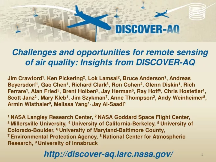
Challenges and opportunities for remote sensing of air quality: Insights from DISCOVER-AQ.

E N D
Challenges and opportunities for remote sensing of air quality: Insights from DISCOVER-AQ Jim Crawford1, Ken Pickering2, Lok Lamsal2, Bruce Anderson1, Andreas Beyersdorf1, Gao Chen1, Richard Clark3, Ron Cohen4, Glenn Diskin1, Rich Ferrare1, Alan Fried5, Brent Holben2, Jay Herman6, Ray Hoff6, Chris Hostetler1, Scott Janz2 , Mary Kleb1, Jim Szykman7, Anne Thompson2, Andy Weinheimer8, Armin Wisthaler9, Melissa Yang1, Jay Al-Saadi1 1 NASA Langley Research Center, 2 NASA Goddard Space Flight Center, 3 Millersville University, 4 University of California-Berkeley, 5 University of Colorado-Boulder, 6 University of Maryland-Baltimore County, 7 Environmental Protection Agency, 8 National Center for Atmospheric Research, 9 University of Innsbruck http://discover-aq.larc.nasa.gov/
Thanks to Partners Maryland Department of the Environment (MDE) San Joaquin Valley Air Pollution Control District (SJV APCD) California Air Resource Board (CARB) Bay Area Air Quality Management District (BAAQMD) Texas Commission on Environmental Quality (TCEQ) Colorado Department of Public Health and Environment (CDPHE) Environmental Protection Agency, Office of Res. and Dev. National Center for Atmospheric Research National Science Foundation National Oceanic and Atmospheric Administration National Park Service University of Maryland, College Park; Howard University University of California, Davis; University of California, Irvine University of Houston; Rice University; University of Texas; Baylor University; Princeton University of Colorado-Boulder; Colorado State University
Investigation Overview Deriving Information on Surface Conditions from Column and VERtically Resolved Observations Relevant to Air Quality A NASA Earth Venture campaign intended to improve the interpretation of satellite observations to diagnose near-surface conditions relating to air quality Objectives: 1. Relate column observations to surface conditions for aerosols and key trace gases O3, NO2, and CH2O 2. Characterize differences in diurnal variation of surface and column observations for key trace gases and aerosols 3. Examine horizontal scales of variability affecting satellites and model calculations
Deployment Strategy Systematic and concurrent observation of column-integrated, surface, and vertically-resolved distributions of aerosols and trace gases relevant to air quality as they evolve throughout the day. Three major observational components: NASA UC-12 (Remote sensing) Continuous mapping of aerosols with HSRL and trace gas columns with ACAM NASA P-3B (in situ meas.) In situ profiling of aerosols and trace gases over surface measurement sites Ground sites In situ trace gases and aerosols Remote sensing of trace gas and aerosol columns Ozonesondes Aerosol lidar observations
Deployment Locations Maryland, July 2011 Houston, September 2013 Colorado, Jul-Aug 2014 California, Jan-Feb 2013
Predicted NO2 Column Behavior Taken from Fishman et al., BAMS, 2008
Predicted NO2 Column Behavior NO2:NOx NO2 Column Photochemical Loss Emissions Taken from Boersma et al., JGR, 2008
Pandora Statistics-Maryland 1 x 10¹⁵ mol/cm2 = 0.037 DU Median and inner quartile values plotted
Pandora Statistics-Houston 1 x 10¹⁵ mol/cm2 = 0.037 DU Median and inner quartile values plotted
Pandora Statistics-California 1 x 10¹⁵ mol/cm2 = 0.037 DU Median and inner quartile values plotted
P-3B Profile Statistics-CaliforniaUrban sites: Bakersfield+Fresno
Pandora Statistics-Colorado 1 x 10¹⁵ mol/cm2 = 0.037 DU Median and inner quartile values plotted
Summary • 1. DISCOVER-AQ has collected a dataset of unprecedented detail on the diurnal trends in air quality as it is discerned from in situ and remote sensing methods. • 2. NO2 columns exhibit both unexpected and diverse diurnal trends that are consistent with vertically resolved profiles. • 3. NO2 tropospheric column retrievals are highly sensitive to diurnal variation in a-priori profile shapes. • 4. Next analysis steps include looking beyond median statistics.
Implications for TEMPO (1 of 2) • An airborne validation campaign is probably beyond TEMPO’s budget • D-AQ core budget $30M for 5-year, 4-campaign study; partner contributions added ~$10M • Typical R&A-directed campaign budgets $15-$20M (3-yr total) • 1-month GeoTASO/GCAS deployment ~$1M for flights & data processing • There’s no guarantee that an R&A airborne campaign will take place over North America during TEMPO prime mission • NASA R&A led airborne campaigns for atmospheric composition historically occur every 2-4 years; have to take turns with other science focus areas • Competing resource demands, within atmospheric composition and with EV-S
Implications for TEMPO (2 of 2) • So what do we do? • Science studies related to TEMPO observations are a logical priority for tropospheric chemistry programs post-launch • Analysis of DISCOVER-AQ, KORUS-AQ, TROPOMI and other data sets will help clarify priorities for pre- & post-launch airborne campaigns related to TEMPO • Spatial representativeness, diurnal influences on products, vertical profile shapes, … • Get in line and build advocacy: NASA campaign concepts typically start as community grass-roots efforts leading to development of white papers • Consider Earth Venture proposal? • Continue preparatory activities as funding permits (GEO-CAPE, HQ R&A, possibly HQ Applied Science, possibly TEMPO)
Thoughts from Jim Crawford on Possible Approaches • There are at least two initial approaches to take. • One is to leverage what we have learned from DISCOVER-AQ, KORUS-AQ, etc. to define a field campaign to support TEMPO. In this case, you would hope to be able to get airborne as soon as possible after TEMPO launches. • Another approach would be to get the right surface measurements in place and use them to identify the locations where TEMPO needs the most help. This would delay a field campaign in favor of getting a chance to evaluate TEMPO performance using ground obs, sondes, Pandora, TROPOMI, etc. Such a campaign would hopefully be more targeted on TEMPO performance, but would also hope to see TEMPO observations continue beyond the initial 2-years to take advantage of what is learned.
P-3B Profile Statistics-CaliforniaUrban sites: Bakersfield+Fresno
Observed NO2 Column Behavior Taken from Tzortziou et al., JGR, 2014
Two PBL schemes selected based on the study by Clare Flynn • Emissions and photolysis rate changed based on Anderson et al., 2014 and Canty et al., 2014
Remote Sensing Column Air Mass Factor Sensitivity: Observations and Methods • Location: Padonia, Maryland • Observation period: 3-4 spirals for 14 days in July 2011 (Hours covered 6 AM – 5 PM, local time) • NO2 observations: • Aircraft (P3B) measurements (200 m - ~4 km) NCAR data (accuracy better than10%) • Surface measurements by photolytic converter instrument (accuracy better than 10%) • Spatial resolution comparable between model (4x4km) and spiral (radius ~4km) • Observed PBL heights : Estimation based on temperature, water vapor, O3 mixing ratios, and RH (Donald Lenschow) • Methods: • Model and surface measurements sampled for the days and time of aircraft measurements • Spiral data sampled at model vertical grids
Comparison of NO2 profiles and shape factors • Filled circles: observed grid average • Open circles: linear interpolation in log space • Error bars: standard deviation fi NO2 shape factors Ωi partial column wi scattering weights (VLIDORT) AMF (Observation) = 1.94 AMF (Base) = 2.16 AMF (ACM2 Mod) = 2.3 AMF (YSU Mod) = 1.8
Errors in AMFs/retrievals from a-priori NO2 profiles • AMF calculated for ACAM (air-borne spectrometer located at ~8km) but is also relevant for tropospheric NO2 column retrievals wi scattering weights fi NO2 shape factors • Surface reflectivities: 0.1 to 0.14 at 0.01 steps • Solar zenith angles: 10° to 80° at 10° steps • Aerosol optical depths: 0.1 to 0.9 at 0.1 steps
NO2 profiles and AMFs (11 AM) AMF (Observation) = 1.94 AMF (Base) = 2.16 AMF (ACM2 Mod) = 2.3 AMF (YSU Mod) = 1.8