INTRODUCTION INTO FINITE ELEMENT NONLINEAR ANALYSES

1. INTRODUCTION INTO FINITE ELEMENT NONLINEAR ANALYSES Doc. Ing. Vladimír Ivančo, PhD. Technical University of Košice Faculty of mechanical Engineering Department of Applied Mechanics and Mechatronics HS Wismar, June 2010

2. CONTENS • Introduction • Types of structural nonlinearities • Concept of time curves • Geometrically nonlinear finite element analysis • Incremental – iterative solution • Incremental method • Iterative methods • Material nonlinearities • Examples

3. INTRODUCTION • Sources of nonlinearities • Linear static analysis - the most common and the most simplified analysis of structures is based on assumptions: • static = loading is so slow that dynamic effects can be neglected • linear = a) material obeys Hooke’s law b) external forces are conservative c) supports remain unchanged during loading d) deformations are so small that change of the structure configuration is neglectable

4. Consequences: • displacements and stresses are proportional to loads, principle of superposition holds • in FEM we obtain a set of linear algebraic equations for computation of displacements where K – global stiffness matrix d – vector of unknown nodal displacements F – vector of external nodal forces

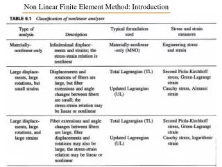
5. Nonlinear analysis – sources of nonlinearities can be classified as • Geometric nonlinearities- changes of the structure shape (or configuration changes) cannot be neglected and its deformed configuration should be considered. • Material nonlinearities - material behaves nonlinearly and linear Hooke’s law cannot be used. More complicated material models should be then used instead e.g. • nonlinear elastic (Mooney-Rivlin’s model for materials like rubber), elastoplastic (Huber-von Mises for metals, Drucker-Prager model to simulate the behaviour of granular soil materials such as sand and gravel) etc. • Boundary nonlinearities - displacement dependent boundary conditions. The most frequent boundary nonlinearities are encountered in contact problems.

6. Consequences of assuming nonlinearities in FEM: Instead of set of linear algebraic equations we obtain a set of nonlinear algebraic equations Consequences of nonlinear structural behaviour that have to be recognized are: • The principle of superposition cannot be applied. For example, the results of several load cases cannot be combined. Results of the nonlinear analysis cannot be scaled.

7. Only one load case can be handled at a time. • The sequence of application of loads (loading history) may be important. Especially, plastic deformations depend on a manner of loading. This is a reason for dividing loads into small increments in nonlinear FE analysis. • The structural behaviour can be markedly non-proportional to the applied load. The initial state of stress (e.g. residual stresses from heat treatment, welding etc.) may be important.

8. b) Concept of time curves In order to reflect history of loading, loads are associated with time curves. Example - values of forces at any time are defined as where f1 and f2 are nominal (input) values of forces and 1 and 1 are load parameters that are functions of time t.

9. For nonlinear static analysis, the “time” variable represents a pseudo time, which denotes the intensity of the applied loads at certain step. For nonlinear dynamic analysis and nonlinear static analysis with time-dependent material properties the “time” represents the real time associated with the loads’ application. The most common case – all loads are proportional to time:

10. 2.Geometrically nonlinear finite element analysis Example – linearly elastic truss

11. Condition of equilibrium axial force where cross-section of the truss engineering strain Initial and current length of the truss are

12. To avoid complications, it is convenient to introduce new measure of strain – Green’s strain defined as In our example is hence

13. Example of different strain measures Logarithmic strain (true strain)

14. The stress-strain relation was measured as When using Green’s strain the relation should be This means that constitutive equation should be

15. The new modulus of elasticity is not constant but it depends on strain If strain is small (e.g. less than 2%) differences are negligible

16. Assuming that strain is small, we can write and after substituting into equation we can derive the condition of equilibrium in the form

17. Consequence of considering configuration changes - relation between load P and displacement u is nonlinear Generally, using FEM we obtain a set of nonlinear algebraic equations for unknown nodal displacementsd

18. 4. Incremental – iterative solution Assumption of large displacements leads to nonlinear equation of equilibrium • For infinitesimal increments of internal and external forces we can write • - tangent stiffness matrix

19. a) Incremental method The load is divided into a set of small increments . Increments of displacements are calculated from the set of linear simultaneous equations

20. a) Iterative methods Newton-Raphson method Suppose that initial displacements d0 are known. The first guess of nodal displacements for load F is calculated by solving set of linear algebraic equations where the tangent stiffness matrix is computed for initial guess d0of displacements that is usually found by linear analysis.

21. Computed displacements d1are then checked by substitution into the most probably not accurate, i.e. the condition is not satisfied are unbalanced nodal forces To improve solution we will do: 1. Compute new tangential stiffness matrix 2. Solve new set of algebraic linear equations 3. Compute an improved solution 4. Check the solution, whether 5. If the condition is not satisfied, steps 1 to 5 are repeated.

22. The iterations are schematically shown in the figure

23. Newton-Raphson method (NR) is often combined with incremental method to take history of loading into consideration

24. Example of non-linear static analysis – bending of the beam, considering elastoplastic material bilinear material model

25. Detail of finite element mesh – SHELL4T elements are colored according to their thickness Both, material and geometric nonlinearities are considered

27. COLLAPSE –inability of the beam to resist further load increase

29. Deflection versus load

30. Danke schön für Ihre Aufmerksamkeit Fragen?