Program unit A

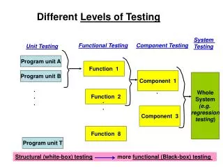
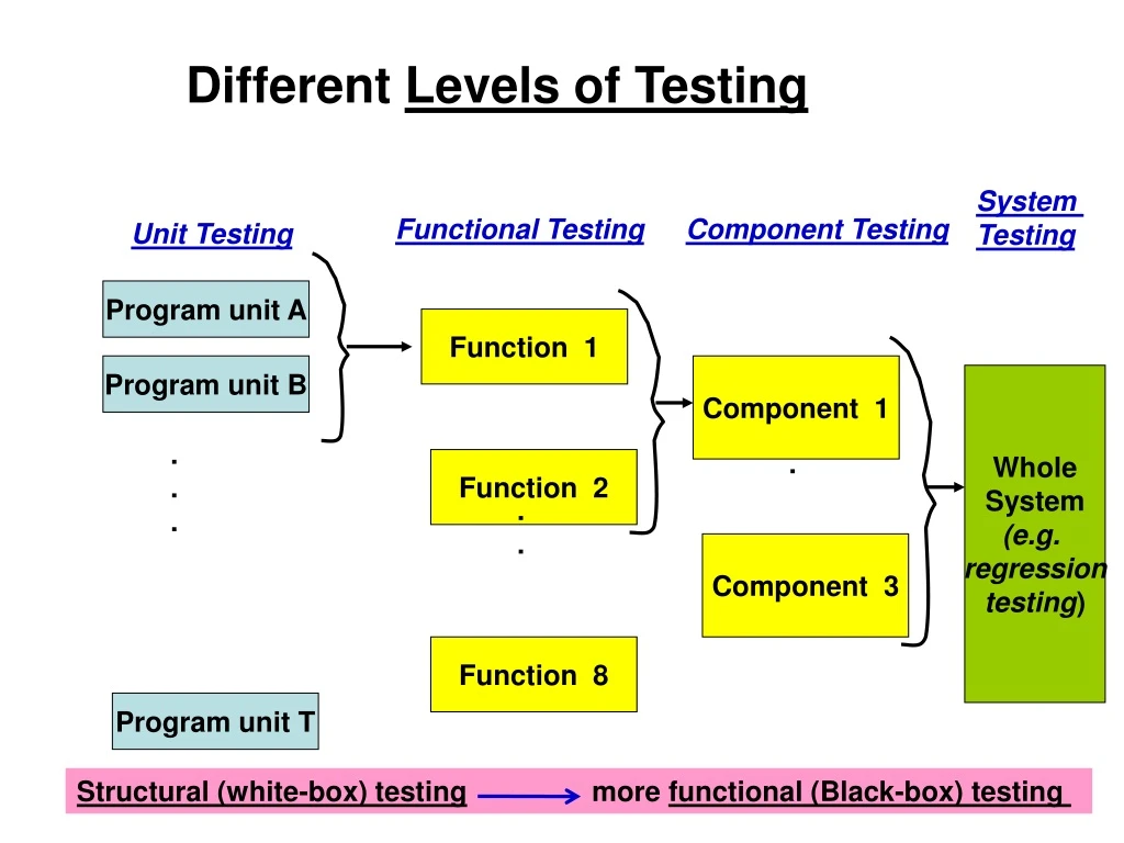
1. Different Levels of Testing System Testing Functional Testing Component Testing Unit Testing Program unit A Function 1 Program unit B Component 1 Whole System (e.g. regression testing) . . . . Function 2 . . Component 3 Function 8 Program unit T Structural (white-box) testing more functional (Black-box) testing

2. Integration Testing • This is the step after the individual pieces of code or modules (programs) are tested. • A set of programs do not exist in vacuum. They are inter-relatedmostly in some manner through: • Calling and passing controls • Calling and passing data or passing “pointers” to data • Integration test looks at the: • “structural” composition (or decomposition) and test the related code (modules / programs). • The “call” relationship neighborhood and test the “neighborhood” • The path created by the relationship and test the “path” Object oriented relationship such as inheritance is addressed differently.

3. Types of Integration tests based onStructural Decomposition • There are 4 major types of integration test for Structural Decomposition Based test: • Top- down • Bottom-up • Combination (Sandwich) • Big Bang

4. Top-down “completed” here means unit tested i) Once the root modules is “completed”, we need to build 3 stubs to perform integration test of root module with stubs. ii) As the next level module is completed, we would build more stubsto perform the next level of integration test iii) Continue this process until all the all the completed modules are tested

5. Bottom-UP i) Once a set of bottom modules are completed we would build a driver, at the next higher level, to run the integration test. ii) Continue this process until all the all the completed modules are tested

6. Combination (Sandwich) If this is completed first, we may choose to build 3 stubs to test - Once a module is completed, we would build the appropriate driver or stubs to perform the integration test. - Continue this process until all the modules are tested “Combo” is a more likely scenario - - - making “integration” management a complex job that needs some tool help. If these two are completed, we may choose to build a driver to test ; may also build two (green) stubs.

7. Big-Bang - Wait for all the modules to be completed and perform one integration (one link-edit). Then test all the integrated modules together. This scenario happens more likely at the over-all system or component test time

8. Some Metrics for Integration Test based on Structural Decomposition • For Top-down approach with n nodes, there is a potential need to construct as much as (n-1) stubs. • For Bottom-up approach with n nodes and v leaves, there is a potential need to construct as much as (n- v)drivers. • For both cases there may be as much as (n – v + edges)number of test sessions (e.g. cases or scenarios)

9. Simple Construct Example for the Metrics A B C D E • There are 5 nodes and 4 leaves and 4 • edges: • n- 1 = 5 -1 = 4 stubs • n - v = 5 - 4 = 1 driver • n - v+ edges = 5 - 4 + 4 = 5 testsessions Number of test sessions = 5: (Top-down) (Bottom-up) 1. A is complete: E is complete: test with 4 stubs test with driver A 2. B is complete: D is complete: test with 3 stubs test with driver A 3. C is complete: C is complete: test with 2 stubs test with driver A 4. D is complete: B is complete: test with 1 stub test with driver A 5. E is complete: A is complete: test all modules test all modules

10. Slightly Modified Example for the Metrics A Number of test sessions = 6: (Top-down) (Bottom-up) 1. A is complete: E is complete: test with 2 stubs test with driver A 2. B is complete: D is complete: test with 2 stubs test with driver B 3. B is complete: C is complete: test with A test with driver B 4. C is complete: B is complete: test with B test with C and D 5. D is complete: B is complete: test with B test with driver A 6. E is complete: A is complete: test all modules test all modules B E C D • There are 5 nodes and 3 leaves and 4 • edges: • n- 1 = 5 -1 = 4 stubs • n - v = 5 - 3 = 2 drivers • n - v+ edges = 5 – 3 + 4 = 6 testsessions

11. One of the key drawbacks to top-down or bottom-up testing for Decomposition-based integration testing is the need for constructing drivers and stub. Pair wiseintegration testing waits for a “related pair”of modules to be completedand then test them. Thus it eliminates the stubs and drivers. There is also a potential reduction in test sessions (# of edges). . Pair-Wise Integration(Sandwich-like) “Related” via edge connection

12. Example of Pair-wise Testing A A B E B C D E C D Pair-wise test sessions : 4 1. A – B 2. B – C 3. B – D 4. A – E Pair-wise test sessions : 4 1. A – B 2. A – C 3. A – D 4. A – E

13. “Neighborhood” Integration Testing • Neighborhood of a node is the set of nodes that are one edge away from the given node. • Thus the neighborhood of a node, n, are all the predecessors and successor nodes of n. • # of neighborhoods = # of interior nodes + source node . • There are some positive and negative characteristics with neighborhood integration testing: • Positives: • Less test sessions • ** Possibly give more of a “behavior” view of a “thread” • Negative: • May be harder to locate bugs • Wait for the completion (timing) of a neighborhood before testing

14. Number of “neighborhoods” • Number of neighborhoods in a call graph may be viewed as: • Number of interior nodes (that form neighborhoods around them) and • 1 neighborhood around the root node • Numerically: • Interior nodes = all nodes – ( source node + sink nodes) • # of Neighborhood = interior nodes + source node • # of Neighborhood = all nodes – sink nodes Note that source node is the 1 root-node in our case: - we should start with the neighborhood around the root - then consider all the neighborhoods around the interior nodes

15. Example of Neighborhood Integration Testing A A B E B C D E C D Total nodes = 5 Sink nodes = 4 Neighborhood = 5 - 4 = 1 Total nodes = 5 Sink nodes = 3 Neighborhood = 5 – 3 = 2 A A A B B E B C D E D C neighborhood(1) (1) neighborhood neighborhood (2)

16. How many neighborhoods are there? A D B C G E H F J I There are ( 10 nodes – 5 sink nodes) = 5 neighborhoods - 1 around the root (start here --- so there is some potential wait time) - 1 around B - 1 around E - 1 around C - 1 around D

17. Path Based Integration Test • Instead of just focusing on the interfaces of the “related” modules in integration test, it would be more meaningful to also focus on the “interactions” among these related modules. • An extension of the neighborhood would be to trace a complete “thread” of interactions among the modules and test that “thread” or “path.”

18. Some Definitions for Path-based Integration Test • Source nodeis the point where program execution starts • Sink nodeis the point where the program execution stops • A module execution pathis a sequence of statements that begins with a source node and ends with a sink node, with no intervening sink nodes. • A message is a “mechanism” with which one unit of code transfers control to another unit of code; control return is also a message • An MM-path (module-to-module path) is an interleaved sequenceof i) module execution paths and ii) messages • Sequence of “nodes” represent a module execution path • Sequence of “edges” represent the messages • An MM-Path Graphis the directed graph in which nodes are from the module execution paths and edges are passing of control/messages.

19. A Simple Example of an MM-Path (Module B) (Module C) (Module A) 1 1 1 2 2 3 2 4 3 3 4 5 6 4 5 Source nodes : A1 and A5 Sink nodes: A4 and A6 Source nodes : B1 and B3 Sink nodes: B2 and B4 Source nodes : C1 Sink nodes: C5 Note: Should modules A and B be recoded ? A1= <1,2,3,6>; A2=<1,2,4> ; A3 = <5,6> Module Execution Paths: B1= <1,2> ; B2 = <3,4> C1= <1,2,4,5> ; C2= <1,3,4,5>

20. Simple Example of MM-Path Graph(from previous slide) A2 B1 A1 C1 B2 C2 A3 - The MM-Path that goes across modules may be looked upon as an inter-module “slice.” - In large and medium sized systems, an MM-Path may be viewed as a “major application function/thread”.