Download
1 / 60
600 likes | 1k Views
Linkage, genetic maps. Macular degeneration is a group of diseases characterized by a breakdown of the macula. The macula is the center portion of the retina that makes central vision and visual acuity possible.

E N D
Macular degeneration is a group of diseases characterized by a breakdown of the macula. The macula is the center portion of the retina that makes central vision and visual acuity possible. “Age-related maculopathy (ARM), also known as age-related macular degeneration (AMD), is the leading cause of irreversible vision loss in the elderly population in the USA and the Western world and a major public health issue. Affecting nearly 9% of the population over the age of 65, ARM becomes increasingly prevalent with age such that by age 75 and older nearly 28% of individuals are affected (1–6). As the proportion of the elderly in our population increases, the public health impact of ARM will become even more severe. Currently there is little that can be done to prevent or slow the progression of ARM (7).” http://hmg.oupjournals.org/cgi/content/full/9/9/1329#DDD140TB1
Hmmmmm “It was not long from the time that Mendel's work was rediscovered that new anomalous ratio began appearing. One such experiment was performed by Bateson and Punnett with sweet peas. They performed a typical dihybrid cross between one pure line with purple flowers and long pollen grains and a second pure line with red flowers and round pollen grains. Because they knew that purple flowers and long pollen grains were both dominant, they expected a typical 9:3:3:1 ratio when the F1 plants were crossed. The table shows the ratios that they observed. Specifically, the two parental classes, purple, long and red, round, were overrepresented in the progeny.” http://www.ndsu.edu/instruct/mcclean/plsc431/linkage/linkage1.htm
“Coupling” and “repulsion” http://www.ndsu.edu/instruct/mcclean/plsc431/linkage/linkage1.htm
Tests of significance The χ2 test of “goodness of fit” (Karl Pearson)
Classical problem “No one can tell which way a penny will fall, but we expect the proportions of heads and tails after a large number of spins to be nearly equal. An experiment to demonstrate this point was performed by Kerrich while he was interned in Denmark during the last war. He tossed a coin 10,000 times and obtained altogether 5,067 heads and 4,933 tails.” MG Bulmer Principles of Statistics
Hypothesis vs. observation Hypothesis: the probability of getting a tail is 0.5. Observation: 4,933 out of 10,000. Well?!! How can we meaningfully – quantitatively – construct a test that would tell us, whether the hypothesis is, most likely, correct, and the deviation is due to chance – or (alternatively) – the hypothesis is incorrect, and the coin dislikes showing its “head” side for some mysterious reason? Sampling errors are inevitable, and deviations from perfection are observed all the time. The goodness of fit test has been devised to tell us, how often the deviation we have observed could have taken place solely due to chance.
The procedure Come up with an explanation for the data (“the null hypothesis”). Ask yourself – if that explanation were correct, what should the data have been? E.g., if the hypothesis is that the probability of getting “tails” is 50%, then there should have been 5,000 tails and 5,000 heads. This set of numbers forms the “expected data.” Take the actual – observed – data (critical point: take the primary numbers, not the frequencies or percentages – this is because the “goodness of fit” is a function of the absolute values under study). Plug them into the following formula:
Calculate p value. If it’s .05 or below, the hypothesis is incorrect – the deviation you see in the data is unlikely to be due to chance. If it’s above .05, the hypothesis stands.
SMI? Take a pure-breeding agouti mouse and cross it to a pure-breeding white mouse. Get 16 children: all agouti (8 males, 8 females). Cross each male with one female (randomly). Get 240 children in F2: 175 agouti and 65 white (ratio: 2.692).
“End of Drug Trial Is a Big Loss for Pfizer” Dec. 4 2006 The news came to Pfizer’s chief scientist, Dr. John L. LaMattina, as he was showering at 7 a.m. Saturday: the company’s most promising experimental drug, intended to treat heart disease, actually caused an increase in deaths and heart problems. Eighty-two people had died so far in a clinical trial, versus 51 people in the same trial who had not taken it. Within hours, Pfizer, the world’s largest drug maker, told more than 100 trial investigators to stop giving patients the drug, called torcetrapib. Shortly after 9 p.m. Saturday, Pfizer announced that it had pulled the plug on the medicine entirely, turning the company’s nearly $1 billion investment in it into a total loss. The abrupt decision to discontinue torcetrapib was a shocking disappointment for Pfizer and for people who suffer from heart disease. The drug, which has been in development since the early 1990s, raises so-called good cholesterol, and cardiologists had hoped it would reduce the buildup of plaques in blood vessels that can cause heart attacks. Just last Thursday, Pfizer’s chief executive, Jeffrey B. Kindler, said publicly that the drug could be among the most important new developments for heart disease in decades and that the company hoped to get Food and Drug Administration approval for it in 2007. “I’m terribly disappointed,” said Dr. Steven E. Nissen, chairman of cardiovascular medicine at the Cleveland Clinic and lead investigator of an earlier torcetrapib clinical trial. “This drug, if it worked, would probably have been the largest-selling pharmaceutical in history.”
Back to Bateson and Punnett What is going on? What can explain this “repulsion and coupling”? Why are these two genes disobeying Mendel’s second law?
Morgan’s observation of linkage One of these genes affects eye color (pr, purple, and pr+, red), and the other affects wing length (vg, vestigial, and vg+, normal). The wild-type alleles of both genes are dominant. Morgan crossed pr/pr · vg/vg flies with pr+/pr+ · vg+/vg+ and then testcrossed the doubly heterozygous F1 females: pr+/pr · vg+/vg × pr/pr · vg/vg .
The data 1:1:1:1?!
These two loci do not follow Mendel’s second law because they are linked
The data ?
Unit definition 1% recombinant progeny = 1 map unit = 1 centimorgan (cM) ~ 1 Mb (note: the latter applies to humans)
If genes are more than 50 map units apart, they behave as if they were unlinked.
Bridges (left) and Sturtevant in 1920. G. Rubin and E. Lewis Science 287: 2216.
The three-point testcross From my perspective, the single most majestic epistemological accomplishment of “classical” genetics
Reading Two chapters from Morgan’s book (III, on linkage, and V, on chromosomes). A short chapter from Sturtevant’s History of Genetics. Chapter 5, section 2.
How to Map Genes Using a Three-Point Testcross • Cross two pure lines. • Obtain large number of progeny from F1. • Testcross to homozygous recessive tester. • Analyze large number of progeny from F2.
v+/v+ · cv/cv · ct/ctv/v · cv+/cv+ · ct+/ct+. v/v+ · cv/cv+ · ct/ct+ v/v · cv/cv · ct/ct. P F1 Two Drosophila were mated: a red-eyed fly that lacked a cross-vein on the wings and had snipped wing edges to a vermilion-eyed, normally veined fly with regular wings. All the progeny were wild type. These were testcrossed to a fly with vermilion eyes, no cross-vein and snipped wings. 1448 progeny in 8 phenotypic classes were observed. Map the genes.
2. Rewrite data Arrange in descending order, by frequency. NCOs DCOs
3. Determine gene order With the confusion cleared away, determine gene order by comparing most abundant classes (non-recombinant, NCO) with double-recombinant (least abundant, DCO), and figuring out, which one allele pair needs to be swapped between the parental chromosomes in order to get the DCO configuration. This one allele pair will be of the gene that is in the middle.