1 Institute of Applied Physics, J. Kepler University, Linz, Austria

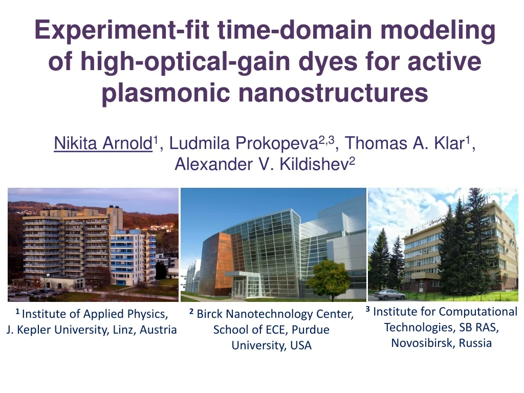
1. Experiment-fit time-domain modeling of high-optical-gain dyes for active plasmonic nanostructuresNikita Arnold1, Ludmila Prokopeva2,3, Thomas A. Klar1, Alexander V. Kildishev2 3 Institute for Computational Technologies, SB RAS, Novosibirsk, Russia 1Institute of Applied Physics, J. Kepler University, Linz, Austria 2 Birck Nanotechnology Center, School of ECE, Purdue University, USA

2. Why model dyes in nano-plasmonics? 2 Experimental proof: high losses require high gain: lossless fishnet with Rh8002 H • Numerical requirements: • Unified description for dispersion and gain • Algorithms: minimize flops, scalability, parallelization, stability, accuracy • Applicable to FDTD (structured mesh), FVTD and FETD (shape-conformal unstructured meshes) • Aims of detailed modeling: • Experiments, new physics, devices • Challenges: • Dispersion, population dynamics • Multiphysics: saturation, NL effects, e-phonons-T, phase changes, chemistry, etc. - all evolve in time X Y Time domain Numerical issues are scarcely addressed in literature3,4 Limiting factor: losses. Proposal: fight losses with gain1 Silver Al2O3 Gain material 1Klar, Kildishev, Drachev, Shalaev, IEEE J. of Sel. Top. in Quant. Electr. 12, 1106 (2006) 2Xiao, Drachev,Kildishev, Ni, Chettiar, Yuan, Shalaev, Nature 466, 735 (2010) 3Trieschmann , Xiao , Prokopeva, Drachev, Kildishev, Opt. Express19(19) 18253 (2011) 4Prokopeva, Bornemann, Kildishev, IEEE Trans. Magn.47(5), 1150 (2011)

3. Dispersion: from a Pade approximant to physical terms Frequency-Domain Drude Conductivity Debye Lorentz, Sellmeier, CP () - arbitrary Pade Partial fraction decomposition Time-Domain aj– amplitude, j – phase, δj –oscillation, γj – damping Simple terms in p(t)=()*E(t-) convolution are calculated recursively

4. Dispersion: Universal time-domain implementation Invert () terms  Auxiliary Differential Equations (ADE): Drude, Debye, Lorentz, Sellmeier, Critical Point (CP) Recursive Convolution (RC) n-kEk with k=ck-1 ≈ 1 = Finite-Difference (FD) approximation Different RC approx. lead to different FD schemes Similar FD Equations for both ADE and RC. 2-3 stencil, 2nd order ■ all Models in one framework ■ less parameters ■ less flops (>30%) Dispersion section is published in IEEE Trans. Magn. (2011) 47-5

5. From dispersion to gain Lorentzian example: 4 level scheme for Rh800 3 32~0.3ps 2 pumping, K30~29ns 695 nm, 30~9fs lasing, K21~6.3ns 723 nm, 21~3.75fs nr21~262ps r21~6.3ns 1 10~0.35ps 0 Polarizations: Lorentz oscillators with N(t) Full p-N system Populations dynamics Fast driving terms (energy exchange) Full p-N: Siegman, Lasers, (1986); DM: Rautian, Shalagin, Kinetic Problems of Nonlinear Spectroscopy (1991) AND Boyd, Nonlinear Optics (2008); Polarizations are coupled to Maxwell’s equations

6. pulse=2ps pump=695nm probe=720nm Result: All parameters are close to methanol values, apart from  Chemical environment affects NR lifetimes nr,212 0.77ns nr,21 0.26ns Parameters retrieval for gain medium1 Simulations: 4-level p-N scheme + 1D Maxwell • Different pulse durations (time dynamics) • Different wavelengths (spectral behavior) • RMS fitting for probe=720nm model parameters • Key parameter: r,21+ measured  • Experiment: dependence of probe transmission on pump intensity • Rh800 in epoxy solid film. No literature values (only e.g., methanol host2) • Pump-probe: • Different probe (703…726nm) • Different pulse (103fs, 2ps) • Rh800/ethanol reference for quantum yield  1Trieschmann , Xiao , Prokopeva, Drachev, Kildishev, Opt. Express 19(19) 18253 (2011) 2D. P. Benfey et al., “Diode-pumped dye laser analysis and design”, Applied Optics 31, 7034 (1992)

7. Levels of description: QM: ( or ), Full p-N, SVEA, Rateequations, () Energy exchange Complex SVEs Full p-N SVEs SVEA Rate Lorentzian absorption/emission SVEA: average over Tlight, always works, is ~101-2 times faster Rate equations: fail for short pulses, coherent effects

8. Examples of Rh800 dynamicsand () recovery Polarizabilities 0.02 0.01 gain 3 0 0 Real analytical -0.01 -0.02 0.04 0.03 Lorentzian ”30absorption Imag 0.02 0.01 0 650 660 670 680 690 700 710 720 730 740 750 wavelength, nm Polarizabilities E=109V/m 0.02 0.01 30 saturation 0 Real -0.01 gain 3 0 analytical post-pulse 21 inversion -0.02 0.04 ”30 saturates 0.03 0.02 Imag 0.01 0 650 660 670 680 690 700 710 720 730 740 750 wavelength, nm =10fs, 30abs=695nm E=108V/m - “weak” field

9. Coherent effects for 30 transition in Rh800 3 32~0.3ps 2 pumping, K30~29ns 695 nm, 30~9fs lasing, K21~6.3ns 723 nm, 21~3.75fs r21~6.3ns nr20~262ps 1 10~0.35ps 0 Rabi terms =50fs, 30abs=695nm E=109V/m (I=2.21011W/cm2) Coherent 30 inversion 32 relaxation 21 inversion

10. All 4 levels are needed to describe high-I absorption 10 3 32~0.3ps 2 pumping, K30~29ns 695 nm, 30~9fs lasing, K21~6.3ns 723 nm, 21~3.75fs r21~6.3ns nr20~262ps 1 10~0.35ps 0 1 N N 0.27 3 3 N N 2 0.8 2 N 0.26 N 1 1 N N 0.6 0 0 0.25 0.4 0.24 0.2 0.23 0 10-6 3.465 3.47 3.475 3.48 3.485 3.49 3.495 3.5 0 1 2 3 4 5 6 7 -6 -5 t, ps t, ps x 10 x 10 4 3 P P when 30 is saturated p21(30)>p30 3 2 1 2 1 2 P P 2 3 0 3 0 sum sum 1 1 0 0 -1 -1 -2 -2 -3 -4 -3 t, ps 3.465 3.47 3.475 3.48 3.485 3.49 3.495 3.5 0 1 2 3 4 5 6 7 Rh800, =1ps, 30abs=695nm E=109V/m (I=2.21011W/cm2) Transition 30: at resonance, saturated Transition 21: off-resonance, inverted, p21(=30) has phase shift Total p=p30+p21<p30,21

11. Complex dyes: beyond single Lorentzian 11 32 31 32 2 lasing K21(1),K21(2) pumping K3(1)0, K3(2)0 nr20 12 11 10 0 • Asymmetric Lorentzians (CP models), virtual levels for MP absorption1 Realistic models should include: • N(t)-saturation, coherent effects (Rabi) • Multilevels, vibronic sub-lines with spectral “mirroring” • Which  to keep? Physics: non-radiative relaxations to vibronic bottoms, radiative “vertical” Do we need such details? • To pinpoint plasmonic resonances • To quantify modifications of dye parameters by metals (Purcell effect, etc.) 1SPIE Proc. (2011) 8172-10

12. 6-level scheme example: “Thermo Scientific Green Fluorescent Dye” in PS film 12 513 1 =438 1 466 0.61 486 0.59 HWHM 4.7, 12fs HWHM 11, 5.3, 8fs 555 0.17 32 31 32~1ps r3(1)0, K3(1)0~55ns, 466nm pumping 2 r3(2)0,K3(2)0~13ns, 438nm K21(1)~84ns, 486nm lasing K21(2)~23ns, 513nm nr20~2.9ns r21(1)~84ns r21(2)~23ns 12 11 10~1ps 0 Experiment (Dr. B. Ding): τfluor = 2.53ns, σabs10-16cm2, =0.14, n“=0.01 (OD @2), =2.3103 cm-1, Ntot=2.3 1019 cm-3

13. (),()-recovery for 6 level scheme. 3fs pump-probe pulses Polarizabilities 0.015 N3 0.2 2 0.01 ’ N3 1 0.15 0.005 N2 Real 0.1 N1 0 del=2ps 2 0.05 N1 -0.005 1 <analyt -saturation N0 0 -0.01 0.02 0 0.5 1 1.5 2 2.5 t, ps -4 x 10 2 sum 0.015 sum gain3 0 2 1 P3 0 pump 2 Imag 0.01 gain3 0 1 P3 0 320=438nm 2109 V/m 0 1 analytical 0.005 P21 ” -1 2 P21 0 1 400 420 440 460 480 500 520 540 560 580 600 -2 0 0.5 1 1.5 2 2.5 wavelength, nm t, ps -5 x 10 5 Polarizabilities 0.002 ’ 0.001 212=513nm 109 V/m 0 0 Real -0.001 probe -5 2 2.005 2.01 2.015 2.02 2.025 2.03 2.035 2.04 2.045 -0.002 0 -0.001 sum gain21 Imag -0.002 2 ”<0 -inversion gain21 -0.003 1 -0.004 400 420 440 460 480 500 520 540 560 580 600 wavelength, nm • Fine spectral structure • All polarizations (lines overlap)  recover separate terms • Frequency scan for longer pulses

14. 6 level scheme, 4m slab. Full p-N+1D Maxwell, pulse=50 fs Probe R, T, Aas a function of pump-probe delay probe=486nm weaker line probe=513nm main line • Pump: E=3109V/m, pump=438nm (main line), Probe: E=107V/m • delay dependence reflects relaxation times 3(1,2)2=1ps • Both emission sub-lines are inverted (A<0), but: • T(513) is amplified (T>1), while T(486) is only enhanced (T>Tno pump) • For ns delay the depopulation of upper emission level 2 settles in

15. 6 level scheme, 4m slab. Full p-N+1D Maxwell, pulse=50 fs Probe R, T, Aas a function of pump intensity probe=513nm main line probe=486nm weaker line • Pump: 109<E<1010V/m (pump=438nm), delay=5ps, Probe: E=107V/m • Fabry-Perot and other 1D effects are important in R,T,A() • T(513) is inverted (A<0) and amplified (T>1) at lowerEpump than T(486): 486nm is weaker and has stronger absorption overlap • Epump dependence reflects saturation fluence • for 320 absorption:

16. Summary Unified numerical modeling of dispersive media IEEE Trans. Magn. (2011) 47-5 Dispersion Unified modeling of gain media - parameter retrieval for gain media - asymmetric Lorentzian line shapes - arbitrary multilevel (ML) schemes Opt. Express (2011) 19(19):18253-9 Gain I SPIE Proc. (2011) 8172-10 Description levels: Full p-N system, SVEA, Rate eqns., coherent and ML effects 6-level system example: ()-recovery, pump-probe transmission dependence on delay, Epump Not published Gain II

17. Funding: ERC grant Active NP 257158 ARO MURI award 50342-PH-MUR ONR MURI grant N00014-10-1-0942 AFRL Materials and Manufacturing Directorate Applied Metamaterials Program Thank you for your attention