Download
1 / 31
340 likes | 585 Views
BRISK (Presented by Josh Gleason). Binary Robust Invariant Scalable Keypoints Sefan Leutenegger , Margarita Chli and Roland Y. Siegwart ICCV11. Overview. Objective Related Work Key-point detection Key-point description Key-point matching Experiments and Results Examples. Objective.

E N D
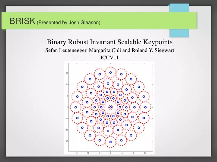
BRISK (Presented by Josh Gleason) Binary Robust Invariant Scalable Keypoints SefanLeutenegger, Margarita Chli and Roland Y. Siegwart ICCV11
Overview Objective Related Work Key-point detection Key-point description Key-point matching Experiments and Results Examples
Objective Detect features which, when compared to state-of-the-art methods Perform similarly. Are dramatically more computationally efficient.
Related Work FAST AGAST BREAF DAISY FREAK SURF SIFT
Keypoint detection steps Create scale space Compute FAST score across scale space. Pixel level non-maximal suppression. Compute sub-pixel maximum across patch. Compute continuous maximum across scales. Re-interpolate image coordinates from scale space feature point detection.
Create scale space Scale space representation Each octave is half-sampled from previous octave. is the original image. Each intra-octave is down-sampled such that it is located between and .
FAST Score Computed at each octave and intra-octave separately. Use the FAST detector score s. s is defined for each pixel as the maximum threshold for FAST detection which still considers an image point a corner. The 16 point FAST detector is used which requires 9 consecutive pixels which are sufficiently brighter or darker than the central pixel.
Keypoint detection Special case Intra-octave which has scale is not computed directly. Instead the 8-element fast detector is used on the original image which approximates the upsampling.
Non-maximal suppression Non-maximal suppression is performed on each octave and intra-octave such that score s is maximal within a 3x3 neighborhood Note: Layer is not considered when performing non-maximal suppression. score s is greater than the scales above and below. This comparison is done against the max value in a 3x3 patch in the scale images above and below.
Subpixel maxima and scale selection Using points obtained using non-maximal suppression. 2D quadratic function is fit to the 3x3 patch surrounding the pixel and sub-pixel maximum is determined. The same is done for the layer above and below. These maxima are then interpolated using a 1D quadratic function across scale space and the local maximum is chosen as the scale for the feature is found. Selected scale
Keypoint Description Sample pattern of smoothed pixels around feature. Separate pairs of pixels into two subsets, short-distance pairs and long-distance pairs. Compute local gradient between long-distance pairs. Sum gradients to determine feature orientation. Rotate short-distance pairs using orientation. Construct binary descriptor from rotated short-distance pairs.
Sampling pattern Number of samples: N = 60 Points are evenly separated around concentric circles. : Intensity of points smoothed with Gaussian proportional to separation of points on circle. i.e., points on each concentric circle use a different kernel. Avoids aliasing effects Size of pattern based on scale (pattern shown for t=1)
Pattern pairs Set containing all pairs of pixels : size of set is for N=60 Compute two subsets based on distance. is the long-distance pairings : size L = 870 for N = 60 is the short-distance pairings : size S = 512 for N = 60
Pattern pairs Long-distance pairs (870) Unused pairs (388) Short-distance pairs (512)
Local gradient/keypoint orientation Strength of gradient between pairs is computed using Overall keypoint direction vector g is estimated by summing gradients of all pairs in long-distance set. Comment: Should keypoints with weak gradient magnitude be eliminated?
Building descriptor Apply sampling pattern rotated by orientation ,of the keypoint. Use rotated short-distance pairings to build binary descriptor . Each bit in is computed from a pair in , so the descriptor is 512 bits long for N = 60.
Descriptor Properties Rotation invariant. Scale invariant.
Descriptor Matching Hamming distance computed for all pairs between images. Count matching bits between descriptors. Efficient computation because this is simply an XOR operation between two 512 bit strings. Threshold for matching is the number of bits able to be matched.
Implementation notes Use AGAST implementation for computing scores in scale space. Uses SSE2 and SSSE3 to aid in computing scale space pyramid. Computing smoothed pixel intensity is actually done using integral images and box filters with floating point boundries, rather than gaussians. Improved SSE Hamming distance calculator. Lookup tabled of discrete rotated and scaled BRISK pattern versions. Consumes about 40MB of RAM but allows algorithm to more efficiently retrieve values from the sampling pattern.
Experiments 7 datasets All comparisons made against first image in dataset. Datasets contain ground-truth homography used to determine corresponding key-points. Considers any pair of keypoints with descriptor distance below a certain threshold a match.
BRISK Repeatability Repeatability score calculated as ratio between corresponding keypoints and the minimum total number of keypoints visible in both images. A circle proportional to scale around each keypoint match on one image are transformed onto the other image. If the circle and ellipse overlap by more than 50% of the union of the shapes, then a match is determined. Used circle comparable in size to those created by SIFT and SURF.
BRISK Repeatability Compare well to SURF except in transform is not too large.
BRISK vs. BREIF SU-BRISK : Unrotated single scale S-BRISK : Single scale
Timing analysis Easily scalable for faster execution by reducing number of sampling-points Examining only one scale. Omitting pattern rotation step (assuming orientation is always 0)
Demo Video http://www.asl.ethz.ch/people/lestefan/personal/BRISK_demo_web.avi
Future work Explore alternatives to scale-space maxima search of saliency scores to yield higher repeatability while maintaining speed. Analyze BRISK pattern such that information content and robustness is optimized.


![[PDF] Free Download Bird Box By Josh Malerman](https://cdn4.slideserve.com/8124717/slide1-dt.jpg)
![[PDF] Free Download Bird Box By Josh Malerman](https://cdn4.slideserve.com/8130267/slide1-dt.jpg)