Calibration of the Electromagnetic Calorimeter of the CMS detector G. Franzoni

1. Calibration of the Electromagnetic Calorimeter of the CMS detector G. Franzoni University of Minnesota T. Tabarelli de Fatis Università & INFN MilanoBicocca • Calibration definition and targets • Calibrations at start-up • In situ strategy for 2010 • Calibration and stability monitoring

2. Preamble • General concepts to provide context • Pointing to areas that will be elaborated in following talks • Addressing areas where actions are needed

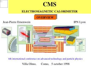
3. High resolution PWO crystal ECAL Barrel: || < 1.48 36 Super Modules 61200 crystals (2 x 2 x 23 cm3) – 26X0 Avalanche photo diodes Endcaps: 1.48 < || < 3.0 4 Dee’s 14648 crystals (3 x 3 x 22 cm3) – 25 X0 Vacuum photo triodes Preshower 3X0 (Pb/Si) 1.65 < |η| < 2.6 ECAL layout • Monitoring in LHC abort gap: • Laser lightinjected in all channels • LED light in endcaps

4. Definitions • Calibration aims at the best estimate of the energy of e/’s • Energy deposited over multiple crystals: • Ee/ = Fe/G iciAi [ +EES ] • Amplitude in ADC counts Ai • Intercalibration: uniform single channel response to a referenceci • Global scale calibration G • Particle-specificcorrections (containment,clustering for e/’s) Fe/ • Preshower included in the sum in endcaps • There’s inter-play across the different terms and a strategy to dis-entangle

5. Status at startup • Precalibrationsci: • Barrel: • 0.3% on 9 SM (electron beams) • 1.5-2.5% on 27 SM (cosmic rays) • ECAL Endcaps: • 6.5% (crystal LY  VPT gain) combined w/ local uniformity of splash events • Still a chance to improve with ES@splash09 • Preshower • 2% (cosmic rays) • Global energyscaleG: • Tied to test beam (also ES) • Corrections: Fe/ • Algorithmic corrections based on MC; η, energy and cluster shape dependent • Need to be tested/tuned in situ since dependent on material budget

6. What if LHC start tomorrow Hγγ width Zee width EB EB EE • Performance acceptable for most physics in EB, nearly in EE • Target: • Target precision: 0.5% set by H benchmark channel • Approach a.s.a.p. in view of resonances

7. Dedicated HLT filters for for fast intercalibrations: -invariance of energy flow within an const-ηring 0/η->γγ mass constraint calibrations with AlCaRaw (RecHits) to increase yield for calibration Both methods provide intercalibration sets in a few days of data taking No need to go into express stream AlcaRaw production and CAF workflows tested at CSA08 and CRAFT09 Performances demonstration still outstanding in endcaps: Worse S/N for 0/η; need ~1 week of data, precision to be assessed Phi-invariance: never reproduced results of CSA06 (1-3%) Fast in situintercalibrationmethods P5 Tier0 CAF AlCaRecoProducers Calibration Algorithms RecHits RawData RecHits HLTFilters

8. In situ strategy • Derive intercalibrations cifrom phi-inv. and 0/η (Marat’s talk) • Fix absolute scale G and corrections (η, ET and cluster shape dependent) Fe/with electrons from Ze+e- (Riccardo’s talk) • ES calibration (mip) and EE-ES inter-calibration (Ming’s talk) • Long-term also other channels: isolated electrons Weν • There’s sufficient redundancy of calibration sources to disentangle interplay between G/Fe/andci: • Validation and combination of calibration sets (tools and procedures in Riccardo’s talk) • Release new sets for reconstruction as long as precision improves. Further sets for monitoring. • Ee/ = Fe/G ici Ai

9. In situ strategy • None of the in situ methods fixes inter-ring scale • ηinter-ring scale and correction functions for ci can be fixed using precalibrations • Inter-ring scale known to better than 0.3% • Ee/ = Fe/G ici Ai 0 calibration

10. ECAL response will vary, depending on dose rate: Crystals transparency drops and recoveries 2010 run: transparency change expected in innermost crystals of EE assuming luminosity will reach L = 1031cm-2s-1 Stability of the ECAL response: transparency Simulation of transparency: η=0.92 @L = 2 x 1033cm-2s-1) Scenario comparable to (ECAL TDR): η=3 @1031cm-2s-1 rel. Crystal response • Transparency variation measured via response R/R0 to blue laser pulses injected in each channel in the LHC abort gap (Adi’s and David’s talks) • Correction to crystal energies proportional to: (R/R0 )α • with α=1.5 BCTP crystals, α=1 SIC crystals

11. VPT gain varies (Sasha’s talk): ‘Classic VPT effect’ induced by LHC on/off changes in cathode current; mitigated by LED constant pulsing to limit current excursions: on average 1% Optimal pulsing strategy yet to be defined Long term ageing: irrelevant in 2010 Stability of the ECAL response:VPT gain Black: load=10kHz, <IC>~0.25nA; 46 days h=2.1 and L=2.5*1033cm2s-1 Grey: load=20kHz, <IC>~1.0nA; 134 days h=2.1 and L=1034cm2s-1 Rel. VPT gain Rel. VPT gain ~25% • Response to blue laser/LED and orangeLED sensitive to VPT gain changes • Correction to crystal energies simply proportional to monitored change (α=1)

12. Calibration and stability • Due to the different values of α, in general one needs to correct separately for transparency and VPT gain: • Ee/ = Fe/G iTiViciAi • Correction for transparency change Ti • Correction for VPT gain change Vi • End-to-end test applying monitoring correction in RECO: yet to be completed • Procedures of validation of monitoring corrections (within start of prompt reco) • Capability of monitoring with orange LED yet to be proven. 2010 data need to establish if LED can provide monitoring of VPT gain alone. • Strategy for 2010: • Activate monitoring procedure based on blue laser only • Being VPT ageing negligible and classic VPT effect ~1%, acceptable using blue laser monitoring to correct for VPT and transparency with the same value of α=1.5

13. Conclusions • Definitions and procedures in place • ECAL calibration at startup: acceptable for most physics analysis • Areas needing attention: • Performance in EE • Stability in EE