Magnet Simulation for NSLS II Lattice Magnets and Insertion Devices.

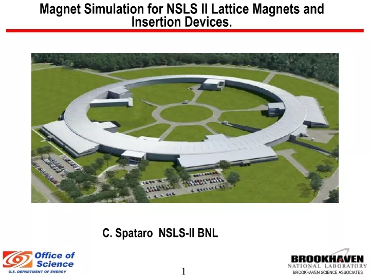
Magnet Simulation for NSLS II Lattice Magnets and Insertion Devices. C. Spataro NSLS-II BNL

Radia & Tosca

RADIA: CPU Efficient 3D Magnetostatics Computer Code Method: Finite Volume Integrals (/ Magnetization Integrals), pioneered in GFUN in 1970s (C.W.Trowbridge et. al.) Origin: European Synchrotron Radiation Facility, first released in 1997 (P.Elleaume, O.Chubar (now@BNL), J.Chavanne) • Features: • Fast analytical calculation of Magnetic Field Strength, Induction and Vector Potential created by Arbitrary Polyhedrons with Uniform Magnetization or / and Current Density over volume; • Fast analytical calculation of infinite Magnetic Field Strength / Induction Integrals along straight lines (important for Accelerator Physics); • Robust Relaxation Scheme ensuring efficient convergence in problems with Fully-Occupied Interaction Matrices and Non-linearIsotropic or Anisotropic Magnetic Materials; • No need to “mesh vacuum” (only active parts of a 3D geometry must be meshed); • Easy Domain Decomposition (“relaxation by parts”); • Support of Space Transformations and Symmetries (plane symmetry, rotation, translation), different types of Boundary Conditions; • Several types of Volume Generators are available, including “generalized extrusion” of a polygon over arbitrary path with translations, rotations and homotheties (including conductors);

NSLS-II Damping Wiggler NdFeB-PM with Side Magnets and Permendur Pole (width 80mm), lu=90mm, Gap=12.5mm • Side • Magnets • End Side • Magnets • Radia v.s. Tosca (0.3% difference in peak By)

Demagnetization Analysis • 0.1mm inside from the gap side • Magnet : Linear anisotropic (permeability in easy direction: 1.06, hard direction : 1.17) Z [mm] • Radia v.s. Tosca

Converting from Radia to Tosca Model • Export .Dxf file from Radia (Mathematica output) • Use Autodesk Inventor to convert dxf to iges file. • Import into Tosca. • Clean up geometry. • Check surface meshing first. • Check volume meshing.

Converting from Radia to Tosca Model 1. Import .dxf file into Autodesk Inventor and save as .igs file

Converting from Radia to Tosca Model 2. Import .igs file into Modeller

Converting from Radia to Tosca Model 3. Create Model body to check model body for errors

Converting from Radia to Tosca Model 3. Generate Surface mesh & Volume mesh to check for meshing errors

Converting from Radia to Tosca Model There were no geometric errors but ...

Converting from Radia to Tosca Model Thin block actually consists of 12 volumes These volumes should be unioned together.

EPU Model – Imported .igs file Converting from Radia to Tosca Model

EPU Model –’Create Model Body’ Error: Converting from Radia to Tosca Model Inconsistent face-body relationship

Epu Model: Deleted 3 Blocks ‘Create Model Body’ now OK Converting from Radia to Tosca Model

Imported 35 mm Dipole .sat File into Modeller Other Modeller Importing Errors Model body created and surface mesh generated.

35 mm Dipole – Volume Mesh Error Other Modeller Importing Errors

35 mm Dipole – Volume mesh error in quadrant Other Modeller Importing Errors

35 mm Dipole – Create Model Body- no errors Other Modeller Importing Errors

35 mm Dipole – Surface mesh- no errors Other Modeller Importing Errors Surface mesh generated

35 mm Dipole – Surface mesh- no errors Other Modeller Importing Errors Zoom of Surface mesh

35 mm Dipole – Surface Mesh Hidden- no errors Other Modeller Importing Errors

Dipole Surface Mesh Hidden Other Modeller Importing Errors This looks to be the problem- surface artifact error found Solution was to delete this quadrant and reflect copy in Z axis

Interaction Study 3 Pole Wiggler &156mm Corrector & 35mm Dipole

Interaction Study 3 Pole Wiggler & 156mm Corrector & 35mm Dipole 35 mm Dipole 156mm Corrector 3 Pole Wiggler 225mm 200mm

Interaction Study 3PW –Dipole-156 mm Dipole Corrector • Model is approximately 3500 mm x 800 mm x 800 mm • Only far field symmetry boundaries are used • Use Block symmetry – set all scale factors=1 • Use current sheets and use them to set the boundary limits in X,Y,& Z

Interaction Studies Current sheets (approx. 50) used to eliminate meshing errors

Interaction Studies More meshing errors in Dipole than either the 3PW or 156mm corrector.

Interaction Study3 Pole Wiggler &156mm Corrector & 35mm Dipole • Large number of nodes (9 x 106) • Long solve time. (This model took 14 days!) • Successful meshing can take longer than the actual solve time- but not in this case. • Counter-intuitive- Start with most complicated model first, ie, one with all components. • This method keeps the background of the model the same (the mesh size, location of the mesh and current sheets etc). • Once meshed- components are then removed one by one and solved.

Interaction Models • 3PW only • 156 mm corrector only • 35 mm dipole only • 3PW + 156 mm Corrector • 3PW + 156 mm corrector + 35 mm dipole

Large Interaction Model (3PW + corrector) model contains the interaction of 3PW and 156 mm corrector. So to get effect of 156 mm corrector on 3PW: =(3PW+ 156mm corrector)-(3PW only) –(156mm only)= effect of 156 MM corrector on 3PW

Magnet Simulation for NSLS II Lattice Magnets and Insertion Devices.