Download

1 / 49
510 likes | 926 Views
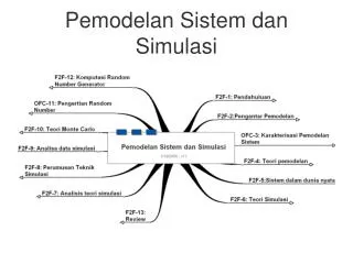
Pertemuan 23 SIMULASI SISTEM. Matakuliah : D0174/ Pemodelan Sistem dan Simulasi Tahun : Tahun 2009. Learning Objectives. Tahapan dalam melakukan simulasi Optimasi Simulasi Simulasi Kalman Filtering Monte Carlo Simulation. Melakukan simulasi. Melakukan simulasi.

E N D
Pertemuan 23SIMULASI SISTEM Matakuliah : D0174/ Pemodelan Sistem dan Simulasi Tahun : Tahun 2009
Learning Objectives • Tahapan dalam melakukan simulasi • Optimasi Simulasi • Simulasi Kalman Filtering • Monte Carlo Simulation
Melakukan simulasi Dilakukan sebagai bagian dari proses rancangan sistem atau pengembangan sistem Alat percobaan menggunakan sebuah model komputer dari sebuah sistem baru/yang ada Melakukan simulasi = sebuah proses dari perancangan model dari sistem nyata dan mengadakan eksperimen dengan model ini 34
Melakukan simulasi konsep sistem model 35
Mulai Formulasi hipotesis Mengembangkan model simulasi Melaksanakan simulasi tidak Proses Hipotesis benar eksperimentasi simulasi ya Selesai 36
Melakukan simulasi Alat evaluasi, BUKAN alat pemecah masalah Memperlihatkan bagaimana sistem bekerja, BUKAN menentukan bagaimana seharusnya dirancang Perpanjangan pikiran yang memungkinkan seseorang mengetahui dinamika yang kompleks dari sebuah sistem, BUKAN pengganti pikiran 37
Definisi Optimasi merupakan proses untuk meningkat performasi model. Model merupakan representasi yang lebih sederhana dari bentuk yang sesungguhnya. Pengembangan model ini akan memudahkan pengguna mengerti tujuan dan peranan model tersebut.
Penentuan Jenis-jenis Performasi Performasi model sangat lah penting untuk dikembangkan, namun ada landasan yang menentukan performasi, yaitu • Kemampuan model untuk membentuk event yang sama dengan sistem nyatanya. • Kemampuan model untuk mencapai tujuan pembuatannya.
Jenis-jenis Optimasi • Estimasi parameter berupa perkiraan terhadap nilai parameter. bagaimana tolak ukur dari tujuan perancangan model tersebut. • Optimasi kebijakan berupa pemilihan beberapa kebijakan untuk memaksimalkan beberapa aspek performansi. model yang dapat digunakan untuk beberapa tujuan yang dapat dipilih.
Nilai Payoff Payoff merupakan proses membandingkan variabel-variabel model dengan data aktual. Jenis-jenis payoff : 1. Payoff kalibrasi 2. Payoff kebijakan(Policy)
Payoff kalibrasi • Berisi nilai-nilai yang dibandingkan dengan nilai bobotnya. • Nilai bobot (E1) di hitung dengan menggunakan rumus berikut : E1=[S-A]/A dimana S : nilai rata-rata hasil stimulasi A : nilai rata-rata data aktual
Contoh Payoff kalibrasi; pada model market.vmf Accrued revenue = unit sales*price Adv budget = frac budget adv*cash revenue Adv impact delay = 12 Demos per person month = 12 Ext sales rep fee = 400 Frac budget mfg = 0.47 Frac budget R and D = 0.15 Int dir sales cost = 2400
Karakteristik Payoff Kalibrasi • Variabel yang akan di validasi - Cash_revenue - Fraction_cust_buying • Format file 1. untuk model market.vmf diperlukan 2 parameter adjustment yaitu produktivitas tenaga sales dan fraksi jumlah costumer yang akan membeli produk jika produknya tersedia.
Karakteristik Payoff Kalibrasi 2. Penentuan parameter disesuaikan dengan tujuan pembentukan model. 3. Nilai parameter payoff kebijakan ditentukan berdasarkan pengetahuan tentang struktur model, dan pemahaman tentang statistik. 4. File disimpan dalam ekstensi.rpm
Payoff Kebijakan(Policy) Kegunaan dari payoff kebijakan adalah untuk menilai performasi sistem. Langkah-langkah : • Definisikan File payoff • Definisikan file Optimasi • Definisikan file changes
Langkah 1; Definisikan File payoff Dalam contoh ini, dimisalkan nama filenya adalah mkt_ppay.prm format penulisannya adalah sebagai berikut *Policy retained_cash_flow /1
Langkah 2; Definisikan file Optimasi Dalam contoh ini, dimisalkan nama filenya adalah mkt_p.prm format penulisannya adalah sebagai berikut 0<=percent_budget_int_dir_sales = 6 <= 50
Langkah 3; Definisikan file change Dalam contoh ini dimisalkan nama filenya adalah mkt_cal.cin normal share of file = 0.88414 demos per person month = 14.4868
DEFINISI Dalam sistem dinamik adakalanya terdapat beberapa variabel yang tidak teramati tetapi diinginkan. Oleh karena itu, jika terdapat beberapa nilai variabel yang diktehui, maka dapat dibuat estimasi beberapa nilai variabel yang lain. Proses inilah yang disebut dengan kalman filtering. Untuk menggunakan ini diperlukan file playoff dan control filter.
Driving noise Driving noise adalah noise dapat mempengaruhi level. Spesifikasi noise menggunkan format sebagai berikut: • Lev_1/0.34/1000 artinya: noise mempengaruhi level 1 memiliki varian 0.34 dan inisial variasi = 1000. nilai variasi merupakan pengukuran ketidak pastian inisial state yang dihitung dari model.
Kontrol simulasi Nilai-nilai yang akan digunakan dalam kalman filtering diperlukan dari data hasil simulasi. Dalam proses simulasi memerlukan file change variabel, yang dalam contoh ini diberi nama wfinv_n.cin. Format penulisannya adalah sebagai berikut: • File wfinv_n.cin inventory meas_noise = 0.4 workforce meas_noise = .025 productivity_noise = .20 net hire noise = 4
Formula variansi σ2 = ∑ (Xi-µ)2/(n-1) n adalah jumlah observasi Xi adalah hasil output
Mekanisme Kalman Filtering • Mengkombinasi data dan model dalam membuat pengukuran secara tidak langsung pada variabel model. • Menggunakan model untuk menciptakan data.
Variansi Noise Dengan menggunakan fungsi random_0_1 (Bilangan random antara 0 dan 1), didapat bilangan random dengan mean 0.5 dan variansi 0.08333 Meas inventory = inventory*(1+(random_0_1)-0.5)*inventory meas noise) Meas workforce = workforce*(1+(random_0_1)-0.5)*workforce meas noise)
What is a Monte Carlo simulation? • In a Monte Carlo simulation we attempt to follow the `time dependence’ of a model for which change, or growth, does not proceed in some rigorously predefined fashion (e.g. according to Newton’s equations of motion) but rather in a stochastic manner which depends on a sequence of random numbers which is generated during the simulation.
Details of the Method • Random Walk: Markov chain is a sequence of events with the condition that the probability of each succeeding event is uninfluenced by prior events • Choosing from Probability Distribution: Any random variable has a probability distribution for its occurrence. We need to choose a random variable which mimics that probability distribution • Best way to relate random number to a random variable is to use cumulative probability distribution and equating it to the random nuber
Random Numbers • Uniformly distributed numbers in [0,1] • Most useful method for obtaining random numbers for computer use is a pseudo random number generator • How random are these pseudo random numbers? Anyone who considers arithmetical methods of producing random digits is, of course, in a state of sin. John von Neumann (1951)
Application to Microscale Heat Transfer • Boltzmann Transport Equation (BTE) for phonons best describes the heat flow in solid nonmetallic thin films • difficult to solve analytically or even numerically using deterministic approaches • alternative is to solve the BTE using stochastic or Monte Carlo techniques
Boltzmann Transport Equation for Particle Transport Distribution Function of Particles: f= f(r,p,t) --probability of particle occupation of momentum p at location rand time t
Equilibrium Distribution: f0, i.e. Fermi-Dirac for electrons, Bose-Einstein for phonons, Plank for photons, etc. Non-equilibrium, e.g. in a high electric field or temperature gradient: Relaxation Time Approximation t Relaxation time
Monte Carlo Solution Technique • Phonons are drawn from the six individual stochastic spaces, including three wave-vector components and the three position vector components • Phonons are then allowed to drift (or unrestrained motion) and scatter in time, and their statistics is collected at various points in time and space, and processed to extract the necessary information
Initial Conditions • number of phonons per unit volume and polarization (p) is usually an extremely large number • a scaling factor is used to simulate only a fraction of the phonons • A series of random numbers properly distributed to match the equilibrium distribution are drawn to initialize the positions, frequencies, polarizations, and wavevectors of the ensemble of phonons chosen for the simulation
Initial conditions • Mazumdar and Majumdar developed a numerical scheme to obtain the number of phonons within the ith frequency interval Dw as:
Boundary Conditions • Isothermal boundary condition: Phonons incident on the wall are removed from the computation domain and a new phonon is introduced in the system which depends on the wall temperature • Adiabatic boundary condition: reflects all the phonons that are incident on the wall
Drift • During the drift phase, phonons move linearly from one location to another and their positions are tracked using an explicit first-order time integration • phonons are tallied within each spatial bin, and the energy of each spatial bin is computed and stored
Scattering • Three-Phonon Scattering (Normal and Umklapp Processes): need to know scattering time-scales, probability of 3-P scattering is given by PNU = 1-exp(-Dt/tNU) • A random number is chosen and compared to the probability, if less then it is scattered • If scattered then the new phonon is generated based on the pseudo temperature of the cell
Scattering • Scattering by Impurities: Scattering by impurities, defects and dislocations are treated in the Monte Carlo scheme in isolation from normal and Umklapp scattering • The time-scale for scattering due to impurities,ti is given by • where a is a constant of the order of unity, r is the defect density per unit volume, and s is the scattering cross-section
2-D Temperature profile Mazumder et al. 2001
Monte Carlo Simulation of Silicon Nanowire Thermal Conductivity • Boundary scattering play an important role in thermal resistance as the structure size decreases to nanoscale
Heat Generation in Electronic Nanostructure Pop E. et al. 2002
Statistical Error • Monte Carlo simulation is a stochastic sampling process, hence have inherent statistical error • errors depend primarily on the number of stochastic samples used in the simulation and the number of scattering events that occur
Daftar Pustaka Kelton, WD., Sadowski, DA, and Sturrock DT. (KS&S). (2003). Simulation with Arena. 3rd edition. McGraw Hill. New York. Harrel. Ghosh. Bowden. (2000). Simulation Using Promodel. McGraw-Hill. New York. Mazumder, S. and Majumdar, A., “Monte Carlo study of phonon transport in solid thin films including dispersion and polarization,” J. of Heat Transfer, vol. 123, pp. 749-759, 2001 Pop E., Sinha S., Goodson K. E., “Monte Carlo modeling of heat generation in electronic nanostructures”, 2002 ASME International Mechanical Engineering Congress and Exposition