Download
1 / 116
1.16k likes | 1.17k Views
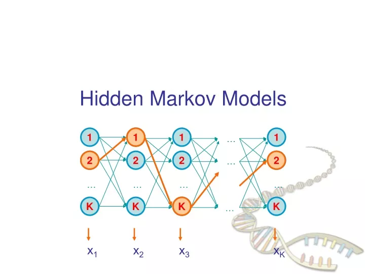
1. 2. 2. 1. 1. 1. 1. …. 2. 2. 2. 2. …. K. …. …. …. …. x 1. K. K. K. K. x 2. x 3. x K. …. Hidden Markov Models. Definition of a hidden Markov model. Definition: A hidden Markov model (HMM) Alphabet = { b 1 , b 2 , …, b M } Set of states Q = { 1, ..., K }

E N D
1 2 2 1 1 1 1 … 2 2 2 2 … K … … … … x1 K K K K x2 x3 xK … Hidden Markov Models
Definition of a hidden Markov model Definition: A hidden Markov model (HMM) • Alphabet = { b1, b2, …, bM } • Set of states Q = { 1, ..., K } • Transition probabilities between any two states aij = transition prob from state i to state j ai1 + … + aiK = 1, for all states i = 1…K • Start probabilities a0i a01 + … + a0K = 1 • Emission probabilities within each state ei(b) = P( xi = b | i = k) ei(b1) + … + ei(bM) = 1, for all states i = 1…K 1 2 K …
A HMM is memory-less At each time step t, the only thing that affects future states is the current state t P(t+1 = k | “whatever happened so far”) = P(t+1 = k | 1, 2, …, t, x1, x2, …, xt) = P(t+1 = k | t) 1 2 K …
The three main questions on HMMs • Evaluation GIVEN a HMM M, and a sequence x, FIND Prob[ x | M ] • Decoding GIVEN a HMM M, and a sequence x, FIND the sequence of states that maximizes P[ x, | M ] • Learning GIVEN a HMM M, with unspecified transition/emission probs., and a sequence x, FIND parameters = (ei(.), aij) that maximize P[ x | ]
Let’s not be confused by notation P[ x | M ]: The probability that sequence x was generated by the model The model is: architecture (#states, etc) + parameters = aij, ei(.) So, P[x | M] is the same with P[ x | ], and P[ x ], when the architecture, and the parameters, respectively, are implied Similarly, P[ x, | M ], P[ x, | ] and P[ x, ] are the same when the architecture, and the parameters, are implied In the LEARNING problem we always write P[ x | ] to emphasize that we are seeking the * that maximizes P[ x | ]
Example: The Dishonest Casino A casino has two dice: • Fair die P(1) = P(2) = P(3) = P(5) = P(6) = 1/6 • Loaded die P(1) = P(2) = P(3) = P(5) = 1/10 P(6) = 1/2 Casino player switches back-&-forth between fair and loaded die once every 20 turns Game: • You bet $1 • You roll (always with a fair die) • Casino player rolls (maybe with fair die, maybe with loaded die) • Highest number wins $2
Question # 1 – Evaluation GIVEN A sequence of rolls by the casino player 1245526462146146136136661664661636616366163616515615115146123562344 QUESTION How likely is this sequence, given our model of how the casino works? This is the EVALUATION problem in HMMs
Question # 2 – Decoding GIVEN A sequence of rolls by the casino player 1245526462146146136136661664661636616366163616515615115146123562344 QUESTION What portion of the sequence was generated with the fair die, and what portion with the loaded die? This is the DECODING question in HMMs
Question # 3 – Learning GIVEN A sequence of rolls by the casino player 1245526462146146136136661664661636616366163616515615115146123562344 QUESTION How “loaded” is the loaded die? How “fair” is the fair die? How often does the casino player change from fair to loaded, and back? This is the LEARNING question in HMMs
The dishonest casino model 0.05 0.95 0.95 FAIR LOADED P(1|F) = 1/6 P(2|F) = 1/6 P(3|F) = 1/6 P(4|F) = 1/6 P(5|F) = 1/6 P(6|F) = 1/6 P(1|L) = 1/10 P(2|L) = 1/10 P(3|L) = 1/10 P(4|L) = 1/10 P(5|L) = 1/10 P(6|L) = 1/2 0.05
1 1 1 1 … 2 2 2 2 … … … … … K K K K … A parse of a sequence Given a sequence x = x1……xN, A parse of x is a sequence of states = 1, ……, N 1 2 2 K x1 x2 x3 xN
1 1 1 1 … 2 2 2 2 … … … … … K K K K … Likelihood of a parse 1 Given a sequence x = x1……xN and a parse = 1, ……, N, To find how likely is the parse: (given our HMM) P(x, ) = P(x1, …, xN, 1, ……, N) = P(xN, N | x1…xN-1, 1, ……, N-1) P(x1…xN-1, 1, ……, N-1) = P(xN, N | N-1) P(x1…xN-1, 1, ……, N-1) = … = P(xN, N | N-1) P(xN-1, N-1 | N-2)……P(x2, 2 | 1) P(x1, 1) = P(xN | N)P(N | N-1) ……P(x2 | 2)P(2 | 1)P(x1 | 1)P(1) = a01 a12……aN-1Ne1(x1)……eN(xN) 2 2 K x1 x2 x3 xN
Example: the dishonest casino Let the sequence of rolls be: x = 1, 2, 1, 5, 6, 2, 1, 6, 2, 4 Then, what is the likelihood of = Fair, Fair, Fair, Fair, Fair, Fair, Fair, Fair, Fair, Fair? (say initial probs a0Fair = ½, a0Loaded = ½) ½ P(1 | Fair) P(Fair | Fair) P(2 | Fair) P(Fair | Fair) … P(4 | Fair) = ½ (1/6)10 (0.95)9 = .00000000521158647211 = 0.521 10-9
Example: the dishonest casino So, the likelihood the die is fair in all this run is just 0.521 10-9 OK, but what is the likelihood of = Loaded, Loaded, Loaded, Loaded, Loaded, Loaded, Loaded, Loaded, Loaded, Loaded? ½ P(1 | Loaded) P(Loaded, Loaded) … P(4 | Loaded) = ½ (1/10)8 (1/2)2 (0.95)9 = .00000000078781176215 = 0.79 10-9 Therefore, it is somewhat more likely that the die is loaded all the way, than that it is fair all the way
Example: the dishonest casino Let the sequence of rolls be: x = 1, 6, 6, 5, 6, 2, 6, 6, 3, 6 Now, what is the likelihood = F, F, …, F? ½ (1/6)10 (0.95)9 = 0.5 10-9, same as before What is the likelihood = L, L, …, L? ½ (1/10)4 (1/2)6 (0.95)9 = .00000049238235134735 = 0.5 10-7 So, it is 100 times more likely the die is loaded
Problem 1: Decoding Find the best parse of a sequence
1 2 2 1 1 1 1 … 2 2 2 2 … K … … … … x1 K K K K … x2 x3 xN Decoding GIVEN x = x1x2……xN We want to find = 1, ……, N, such that P[ x, ] is maximized * = argmax P[ x, ] We can use dynamic programming! Let Vk(i) = max{1,…,i-1} P[x1…xi-1, 1, …, i-1, xi, i = k] = Probability of most likely sequence of states ending at state i = k
Decoding – main idea Given that for all states k, and for a fixed position i, Vk(i) = max{1,…,i-1} P[x1…xi-1, 1, …, i-1, xi, i = k] What is Vl(i+1)? From definition, Vl(i+1) = max{1,…,i}P[ x1…xi, 1, …, i, xi+1, i+1 = l ] = max{1,…,i}P(xi+1, i+1 = l | x1…xi,1,…, i) P[x1…xi, 1,…, i] = max{1,…,i}P(xi+1, i+1 = l | i ) P[x1…xi-1, 1, …, i-1, xi, i] = maxk [P(xi+1, i+1 = l | i = k) max{1,…,i-1}P[x1…xi-1,1,…,i-1, xi,i=k]] = el(xi+1)maxk aklVk(i)
The Viterbi Algorithm Input: x = x1……xN Initialization: V0(0) = 1 (0 is the imaginary first position) Vk(0) = 0, for all k > 0 Iteration: Vj(i) = ej(xi) maxk akj Vk(i-1) Ptrj(i) = argmaxk akj Vk(i-1) Termination: P(x, *) = maxk Vk(N) Traceback: N* = argmaxk Vk(N) i-1* = Ptri (i)
The Viterbi Algorithm x1 x2 x3 ………………………………………..xN Similar to “aligning” a set of states to a sequence Time: O(K2N) Space: O(KN) State 1 2 Vj(i) K
Viterbi Algorithm – a practical detail Underflows are a significant problem P[ x1,…., xi, 1, …, i ] = a01 a12……ai e1(x1)……ei(xi) These numbers become extremely small – underflow Solution: Take the logs of all values Vl(i) = logek(xi) + maxk [ Vk(i-1) + log akl ]
Example Let x be a sequence with a portion of ~ 1/6 6’s, followed by a portion of ~ ½ 6’s… x = 123456123456…123456626364656…1626364656 Then, it is not hard to show that optimal parse is (exercise): FFF…………………...FLLL………………………...L 6 characters “123456” parsed as F, contribute .956(1/6)6 = 1.610-5 parsed as L, contribute .956(1/2)1(1/10)5 = 0.410-5 “162636” parsed as F, contribute .956(1/6)6 = 1.610-5 parsed as L, contribute .956(1/2)3(1/10)3 = 9.010-5
Problem 2: Evaluation Find the likelihood a sequence is generated by the model
1 1 1 1 … 2 2 2 2 … … … … … K K K K … Generating a sequence by the model Given a HMM, we can generate a sequence of length n as follows: • Start at state 1 according to prob a01 • Emit letter x1 according to prob e1(x1) • Go to state 2 according to prob a12 • … until emitting xn 1 a02 2 2 0 K e2(x1) x1 x2 x3 xn
P(box: FFFFFFFFFFF) = (1/6)11 * 0.9512 = 2.76-9 * 0.54 = 1.49-9 P(box: LLLLLLLLLLL) = [ (1/2)6 * (1/10)5 ] * 0.9512 * 0.052 = 1.56*10-7 * 1.5-3= 0.23-9 A couple of questions Given a sequence x, • What is the probability that x was generated by the model? • Given a position i, what is the most likely state that emitted xi? Example: the dishonest casino Say x = 12341623162616364616234161221341 Most likely path: = FF……F However: marked letters more likely to be L than unmarked letters
Evaluation We will develop algorithms that allow us to compute: P(x) Probability of x given the model P(xi…xj) Probability of a substring of x given the model P(I = k | x) Probability that the ith state is k, given x A more refined measure of which states x may be in
The Forward Algorithm We want to calculate P(x) = probability of x, given the HMM Sum over all possible ways of generating x: P(x) = P(x, ) = P(x | ) P() To avoid summing over an exponential number of paths , define fk(i) = P(x1…xi, i = k) (the forward probability)
The Forward Algorithm – derivation Define the forward probability: fk(i) = P(x1…xi, i = k) = 1…i-1 P(x1…xi-1, 1,…, i-1, i = k) ek(xi) = l 1…i-2 P(x1…xi-1, 1,…, i-2, i-1 = l) alk ek(xi) = ek(xi) l fl(i-1) alk
The Forward Algorithm We can compute fk(i) for all k, i, using dynamic programming! Initialization: f0(0) = 1 fk(0) = 0, for all k > 0 Iteration: fk(i) = ek(xi) l fl(i-1) alk Termination: P(x) = k fk(N) ak0 Where, ak0 is the probability that the terminating state is k (usually = a0k)
Relation between Forward and Viterbi FORWARD Initialization: f0(0) = 1 fk(0) = 0, for all k > 0 Iteration: fl(i) = el(xi) k fk(i-1) akl Termination: P(x) = k fk(N) ak0 VITERBI Initialization: V0(0) = 1 Vk(0) = 0, for all k > 0 Iteration: Vj(i) = ej(xi) maxkVk(i-1) akj Termination: P(x, *) = maxkVk(N)
Motivation for the Backward Algorithm We want to compute P(i = k | x), the probability distribution on the ith position, given x We start by computing P(i = k, x) = P(x1…xi, i = k, xi+1…xN) = P(x1…xi, i = k) P(xi+1…xN | x1…xi, i = k) = P(x1…xi, i = k) P(xi+1…xN | i = k) Then, P(i = k | x) = P(i = k, x) / P(x) Forward, fk(i) Backward, bk(i)
The Backward Algorithm – derivation Define the backward probability: bk(i) = P(xi+1…xN | i = k) = i+1…N P(xi+1,xi+2, …, xN, i+1, …, N | i = k) = l i+1…N P(xi+1,xi+2, …, xN, i+1 = l, i+2, …, N | i = k) = l el(xi+1) akl i+1…N P(xi+2, …, xN, i+2, …, N | i+1 = l) = l el(xi+1) akl bl(i+1)
The Backward Algorithm We can compute bk(i) for all k, i, using dynamic programming Initialization: bk(N) = ak0, for all k Iteration: bk(i) = l el(xi+1) akl bl(i+1) Termination: P(x) = l a0l el(x1) bl(1)
Computational Complexity What is the running time, and space required, for Forward, and Backward? Time: O(K2N) Space: O(KN) Useful implementation technique to avoid underflows Viterbi: sum of logs Forward/Backward: rescaling at each position by multiplying by a constant
Posterior Decoding We can now calculate fk(i) bk(i) P(i = k | x) = ––––––– P(x) Then, we can ask What is the most likely state at position i of sequence x: Define ^ by Posterior Decoding: ^i = argmaxkP(i = k | x)
Posterior Decoding • For each state, • Posterior Decoding gives us a curve of likelihood of state for each position • That is sometimes more informative than Viterbi path * • Posterior Decoding may give an invalid sequence of states • Why?
Posterior Decoding x1 x2 x3 …………………………………………… xN • P(i = k | x) = P( | x) 1(i = k) = {:[i] = k}P( | x) State 1 P(i=l|x) l k
Posterior Decoding x1 x2 x3 …………………………………………… xN • Example: How do we compute P(i = l, ji = l’ | x)? fl(i) bl(j) P(i = l, iI = l’ | x) = ––––––– P(x) State 1 P(i=l|x) l P(j=l’|x) k
Viterbi, Forward, Backward VITERBI Initialization: V0(0) = 1 Vk(0) = 0, for all k > 0 Iteration: Vl(i) = el(xi) maxkVk(i-1) akl Termination: P(x, *) = maxkVk(N) FORWARD Initialization: f0(0) = 1 fk(0) = 0, for all k > 0 Iteration: fl(i) = el(xi) k fk(i-1) akl Termination: P(x) = k fk(N) ak0 BACKWARD Initialization: bk(N) = ak0, for all k Iteration: bl(i) = k el(xi+1) akl bk(i+1) Termination: P(x) = k a0k ek(x1) bk(1)
Modeling CpG Islands by HMMs In human genomes the pair CG often transforms to (methyl-C) G which often transforms to TG. Hence the pair CG appears less than expected from what is expected from the independent frequencies of C and G alone. Due to biological reasons, this process is sometimes suppressed in short stretches of genomes such as in the start regions of many genes. These areas are called CpG islands (p denotes “pair”).
CpG Islands • In CpG islands, • CG is more frequent • Other pairs (AA, AG, AT…) have different frequencies Question: Detect CpG islands computationally
Problems: CpG Island We consider two questions (and some variants): Question 1: Given a short stretch of genomic data, does it come from a CpG island ? Question 2: Given a long piece of genomic data, does it contain CpG islands in it, where, what length ? We “solve” the first question by modeling strings with and without CpG islands as Markov Chains over the same states {A,C,G,T} but different transition probabilities:
Question 1: Using two Markov chains A+ (For CpG islands): We need to specify p+(xi | xi-1) where + stands for CpG Island. From Durbin et al we have: Xi Xi-1 (Recall: rows must add up to one; columns need not.)
Question 1: Using two Markov chains A- (For non-CpG islands): …and for p-(xi | xi-1) (where “-” stands for Non CpG island) we have: Xi Xi-1
X1 X2 XL-1 XL Discriminating between the two models Given a string x=(x1….xL), now compute the ratio If RATIO>1, CpG island is more likely. Actually – the log of this ratio is computed: Note: p+(x1|x0) is defined for convenience as p+(x1). p-(x1|x0) is defined for convenience as p-(x1).
Log Odds-Ratio test Taking logarithm yields If logQ > 0, then + is more likely (CpG island). If logQ < 0, then - is more likely (non-CpG island).
Where do the parameters (transition- probabilities) come from ? Learning from complete data, namely, when the label is given and every xi is measured: Source: A collection of sequences from CpG islands, and a collection of sequences from non-CpG islands. Input: Tuples of the form (x1, …, xL, h), where h is + or - Output: Maximum Likelihood parameters (MLE) Count all pairs (Xi=a, Xi-1=b) with label +, and with label -, say the numbers are Nba,+ and Nba,- .
X1 X2 XL-1 XL Where Na,+ is the number of times letter a appear in CpG islands in the dataset. Where Nba,+ is the number of times letter b appears after letter a in CpG islands in the dataset. Maximum Likelihood Estimate (MLE) of the parameters (using labeled data) The needed parameters are: p+(x1), p+ (xi | xi-1), p-(x1), p-(xi | xi-1) The ML estimates are given by:
A model of CpG Islands – Transitions How do we estimate the parameters of the model? Emission probabilities: 1/0 • Transition probabilities within CpG islands Established from many known (experimentally verified) CpG islands (Training Set) • Transition probabilities within other regions Established from many known non-CpG islands
Log Likehoods—Telling “Prediction” from “Random” Another way to see effects of transitions: Log likelihoods L(u, v) = log[ P(uv | + ) / P(uv | -) ] Given a region x = x1…xN A quick-&-dirty way to decide whether entire x is CpG P(x is CpG) > P(x is not CpG) i L(xi, xi+1) > 0