Ch. 7 - QuickSort

1. Ch. 7 - QuickSort Quick but not Guaranteed

2. Ch.7 - QuickSort Another Divide-and-Conquer sorting algorithm… As it turns out, MERGESORT and HEAPSORT, although O(n lg n) in their time complexity, have fairly large constants and tend to move data around more than desirable (e.g., equal-key items may not maintain their relative position from input to output). We introduce another algorithm with better constants, but a flaw: its worst case in O(n2). Fortunately, the worst case is “rare enough” so that the speed advantages work an overwhelming amount of the time… and it is O(n lg n) on average. 91.404

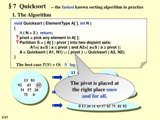
3. Ch.7 - QuickSort Like in MERGESORT, we use Divide-and-Conquer: • Divide: partition A[p..r] into two subarrays A[p..q-1] and A[q+1..r] such that each element of A[p..q-1] is ≤ A[q], and each element of A[q+1..r] is ≥ A[q]. Compute q as part of this partitioning. • Conquer: sort the subarrays A[p..q-1] and A[q+1..r] by recursive calls to QUICKSORT. • Combine: the partitioning and recursive sorting leave us with a sorted A[p..r] – no work needed here. An obvious difference is that we do most of the work in the divide stage, with no work at the combine one. 91.404

4. Ch.7 - QuickSort The Pseudo-Code 91.404

5. Ch.7 - QuickSort 91.404

6. Ch.7 - QuickSort Proof of Correctness: PARTITION We look for a loop invariant and we observe that at the beginning of each iteration of the loop (l.3-6) for any array index k: • If p ≤ k ≤ i, then A[k] ≤ x; • If i+1 ≤ k ≤ j-1, then A[k] > x; • If k = r, then A[k] = x. • Ifj ≤ k ≤ r-1, then we don’t know anything about A[k]. 91.404

7. Ch.7 - QuickSort The Invariant • Initialization. Before the first iteration: i=p-1, j=p. No values between p and i; no values between i+1 and j-1. The first two conditions are trivially satisfied; the initial assignment satisfies 3. • Maintenance. Two cases • 1.A[j] > x. • 2. A[j] ≥ x. 91.404

8. Ch.7 - QuickSort The Invariant • Termination. j=r. Every entry in the array is in one of the three sets described by the invariant. We have partitioned the values in the array into three sets: less than or equal to x, greater than x, and a singleton containing x. Running time of PARTITION on A[p..r] is Q(n), where n = r – p + 1. 91.404

9. Ch.7 - QuickSort QUICKSORT: Performance – a quick look. • We first look at (apparent) worst-case partitioning: T(n) = T(n-1) + T(0) + Q(n) = T(n-1) + Q(n). It is easy to show – using substitution - that T(n) = Q(n2). • We next look at (apparent) best-case partitioning: T(n) = 2T(n/2) + Q(n). It is also easy to show (case 2 of the Master Theorem) that T(n) = Q(n lg n). • Since the disparity between the two is substantial, we need to look further… 91.404

10. Ch.7 - QuickSort QUICKSORT: Performance – Balanced Partitioning 91.404

11. Ch.7 - QuickSort QUICKSORT: Performance – the Average Case As long as the number of “good splits” is bounded below as a fixed percentage of all the splits, we maintain logarithmic depth and so O(n lg n) time complexity. 91.404

12. Ch.7 - QuickSort QUICKSORT: Performance – Randomized QUICKSORT We would like to ensure that the choice of pivot does not critically impair the performance of the sorting algorithm – the discussion to this point would indicate that randomizing the choice of the pivot should provide us with good behavior (if at all possible with the data-set we are trying to sort). We introduce 91.404

13. Ch.7 - QuickSort QUICKSORT: Performance – Randomized QUICKSORT And the recursive procedure becomes: Every call to RANDOMIZED-PARTITION has introduced the (constant) extra overhead of a call to RANDOM. 91.404

14. Ch.7 - QuickSort QUICKSORT: Performance – Rigorous Worst Case Analysis Since we do not, a priori, have any idea of what the splits of the subarrays will be, we have to represent a possible “worst case” (we already have an O(n2) bound from the “bad split” example – so it could be worse… although we hope not). The worst case leads to the recurrence T(n) = max0≤q≤n-1(T(q) + T(n – q - 1)) + Q(n), where we remember that the pivot does not appear at the next level (down) of the recursion. 91.404

15. Ch.7 - QuickSort QUICKSORT: Performance – Rigorous Worst Case Analysis We have to come up with a “guess” and the basis for the guess is our likely “bad split case”: it tells us we cannot hope for any better than W(n2). So we just hope it is no worse… Guess T(n) ≤ cn2 for some c > 0 and start doing algebra for the induction: T(n) ≤ max0≤q≤n-1(T(q) + T(n – q - 1)) + Q(n) ≤ max0≤q≤n-1(cq2 + c(n – q - 1)2) + Q(n). Differentiate cq2 + c(n – q - 1)2 twice with respect to q, to obtain 4c > 0 for all values of q. 91.404

16. Ch.7 - QuickSort QUICKSORT: Performance – Rigorous Worst Case Analysis Since the expression represents a quadratic curve, concave up, it reaches it maximum at one of the endpoints q = 0 and q = n – 1. As we evaluate, we find max0≤q≤n-1(cq2 + c(n – q - 1)2) + Q(n) ≤ c max0≤q≤n-1(q2 + (n – q - 1)2) + Q(n) ≤ c (n – 1)2 + Q(n) = cn2 – 2cn + 1 + Q(n) ≤ cn2 by choosing c large enough to overcome the positive constant in Q(n). 91.404

17. Ch.7 - QuickSort QUICKSORT: Performance – Expected RunTime Understanding partitioning. • Each time PARTITION is called, it selects a pivot element and this pivot element is never included in successive calls: the total number of calls to PARTITION is n. • Each call to PARTITION costs O(1) plus an amount of time proportional to the number of iterations of the for loop. • Each iteration of the for loop (in line 4) performs a comparison , comparing the pivot to another element in A. • We need to count the number of times l. 4 is executed. 91.404

18. Ch.7 - QuickSort QUICKSORT: Performance – Expected RunTime Lemma 7.1. Let X be the number of comparisons performed in l. 4 of PARTITION over the entire execution of QUICKSORT on an n-element array. Then the running time of QUICKSORT is O(n + X). Proof: the observations on the previous slide. We need to find X, the total number of comparisons performed over all calls to PARTITION. 91.404

19. Ch.7 - QuickSort QUICKSORT: Performance – Expected RunTime • Rename the elements of A as z1, z2, …, zn, so that zi is the ith smallest element of A. • Define the set Zij = {zi, zi+1,…, zj}. • Question: when does the algorithm compare zi and zj? • Answer: at most once – notice that all elements in every (sub)array are compared to the pivot once, and will never be compared to the pivot again (since the pivot is removed from the recursion). • Define Xij = I{zi is compared to zj}, the indicator variable of this event. Comparisons are over the full run of the algorithm. 91.404

20. Ch.7 - QuickSort QUICKSORT: Performance – Expected RunTime • Since each pair is compared at most once, we can write • Taking expectations of both sides: • We need to compute Pr{zi is compared to zj}. • We will assume all zi and zj are distinct. • For any pair zi, zj, once a pivot x is chosen so that zi < x < zj, zi and zj will never be compared again (why?). 91.404

21. Ch.7 - QuickSort QUICKSORT: Performance – Expected RunTime • If zi is chosen as a pivot before any other item in Zij, then zi will be compared to every other item in Zij. • Same for zj. • zi and zj are compared if and only if the first element to be chosen as a pivot from Zij is either zi or zj. • What is that probability? Until a point of Zij is chosen as a pivot, the whole of Zij is in the same partition, so every element of Zij is equally likely to be the first one chosen as a pivot. 91.404

22. Ch.7 - QuickSort QUICKSORT: Performance – Expected RunTime • Because Zij has j – i + 1 elements, and because pivots are chosen randomly and independently, the probability that any given element is the first one chosen as a pivot is 1/(j-i+1). It follows that: • Pr{zi is compared to zj} = Pr{zi or zj is first pivot chosen from Zij} = Pr{zi is first pivot chosen from Zij}+ Pr{ zj is first pivot chosen from Zij} = 1/(j-i+1) + 1/(j-i+1) = 2/(j-i+1). 91.404

23. Ch.7 - QuickSort QUICKSORT: Performance – Expected RunTime • Replacing the right-hand-side in 7, and grinding through some algebra: And the result follows. 91.404