Download

1 / 24
240 likes | 248 Views
Workshop 6 Modeling of Catalytic Convertor. Introductory FLUENT Training. Introduction. A workshop to demonstrate how to model porous media in FLUENT

E N D
Workshop 6 Modeling of Catalytic Convertor Introductory FLUENT Training
Introduction • A workshop to demonstrate how to model porous media in FLUENT • Workshop models a catalytic convertor. Nitrogen flows in though inlet with an uniform velocity 22.6 m/s, passes through a ceramic monolith substrate with square shaped channels, and then exits through the outlet. • Substrate is impermeable in Y and Z directions, which is modeled by specifying loss coefficients 3 order higher than in X direction Ceramic Monolith Substrate Inlet Outlet
Starting Fluent in Workbench • Open the Workbench (Start > Programs > ANSYS 12.0 > ANSYS Workbench) • Drag FLUENT into the project schematic • Change the name to Catalytic • Double click on Setup • Choose 3D and Double Precision under Options and retain the other default settings
Import Mesh • Under the File menu select Import> Mesh • Select the file catalytic_converter_125k.msh.gz and click OK to import the mesh • After reading the mesh, check the grid using Mesh>Checkoption or by using CheckunderProblem Setup>General This starts a new Fluent session and the first step is to import the mesh that has already been created:
Setting up the Models • Select Pressure Based, Steady state solver Problem Setup>General>Solver • Specify Turbulence model Problem Setup > Models > Viscous Double click and select k-epsilon (2 eqn) under Model and Realizable under k-epsilon model and retain the default settings for the other parameters • Make sure that the Energy Equation is disabled Problem Setup > Models> Energy
Materials Define the materials. Problem Setup > Materials • Click on air to open Create/Edit Materials panel • Click on FLUENT Database…> Select nitrogen(n2) from the list > Copy • Click on Change/Create
Fluid Zone Conditions • Under Problem Setup >Cell Zone >Double click on part-in under Zone • Select Material Name : nitrogen • Default values for other settings • Click to OK • Similarly, visit to part-outZone and select the same settings as above
Fluid Zone Conditions (2) • Under Problem Setup ->Cell Zone ->Double click on part-catalyst under Zone • Select Material Name : nitrogen • Select and click on Porous Zone • Under Direction-1 Vector, specify as: 1, 0, 0 • Under Direction-2 Vector, specify as: 0, 1, 0 • Specify as per GUI under Viscous Resistance and Inertia Resistance • Default values under Power law Model and Porosity
Operating Conditions • Under Problem Setup >Cell Zone Conditions (operating conditions are also in BC panel) Click on Operating Conditions… and set the Operating Pressure (Pascal) to 101325 pascal
Boundary Conditions Under Problem Setup > Boundary Conditions • Select inlet under Zoneand choose velocity-inlet from the drop down menu under Type • Now double click on inlet under Zone Input all the parameters in Momentum tab as shown below
Boundary Conditions (2) Under Problem Setup > Boundary Conditions • Select outlet under Zoneand choose pressure-outlet from the drop down menu under Type • Now double click on outlet under Zone Input all the parameters in Momentum tab as shown below
Boundary Conditions (3) Under Problem Setup > Boundary Conditions • Wall type boundary condition for the Zone: wall-part-catalyst, wall-part-in and wall-part-out • Interior type of boundary condition for the rest
Solution Methods Under Problem Setup > Solution Methods • SelectCoupledunder Pressure-Velocity Coupling • Select Green-Gauss Node Based under Gradient • Default under other options
Solution Controls Under Problem Setup > Solution Controls • Use default settings
Residual Monitors Residual Monitoring Solution > Monitors Double click on Residuals(By default it is on) Enable Plot under Options. Specify Absolute Criteria for continuity: 1e-4
Surface Monitors Surface Monitors Solution > Monitors > Surface Monitors Monitor points are used to monitor quantities of interest during the solution. They should be used to help judge convergence. In this case you will monitor the Mass Flow Rate atoutletand Static Pressure at inlet.
Initialization Before starting the calculations we must initialize the flow field in the entire domain Solution > Monitors > Solution Initialization • Initializing the flow field with near steady state conditions will result in faster convergence • Select Compute from: inlet • Click on Initialize to initialize the solution
First Order Solution • The solution process can be started in the following manner Solution >Run Calculation • Enter 100 for Number of Iterations and click on Calculate During the iteration process, the residuals and monitor plots will be shown in different windows. You will see that both monitors become flat at 100 iterations. However, this is a solution of first order discretization scheme. To get an accurate solution, we will use higher order discretization scheme for pressure and momentum equations and run further.
Higher Order Solution • Under Solution>Solution Methods setup the parameters as shown below • The solution process can be started in the following manner Solution >Run Calculation • Enter 100 for Number of Iterations and click on Calculate
Convergence history of the solution • Convergence history of the solution can be found from the plots Scaled Residuals Convergence history of Mass Flow Rate on outlet Convergence history of Static Pressure on inlet
Write Case/Data File • To save the project, go to Project Page File>Save as • To write the case/data files, go to FLUENT session File>Export>Case and Data.. Case/Data File: catalytic_converter_second.cas.gz You can now save the project and proceed to write a case file for the solver:
Post Processing • To Draw Contours of Static Pressure on walls Display > Graphics and Animations Double Click on Contours, a new window will pop up Select Pressure under Contours of and Static Pressure below that Select all walls under Surfaces
Post Processing • To get the pressure drop between inlet to outlet boundaries using the porous media model Reports > Surface Integrals Select as per the GUI and click to Compute You will get the information below Hence, the pressure drop is around 734 pascal
Post Processing • You can postprocess any results using the FLUENT postprocessing tools and/or CFD-Post.