Download
1 / 18
180 likes | 300 Views
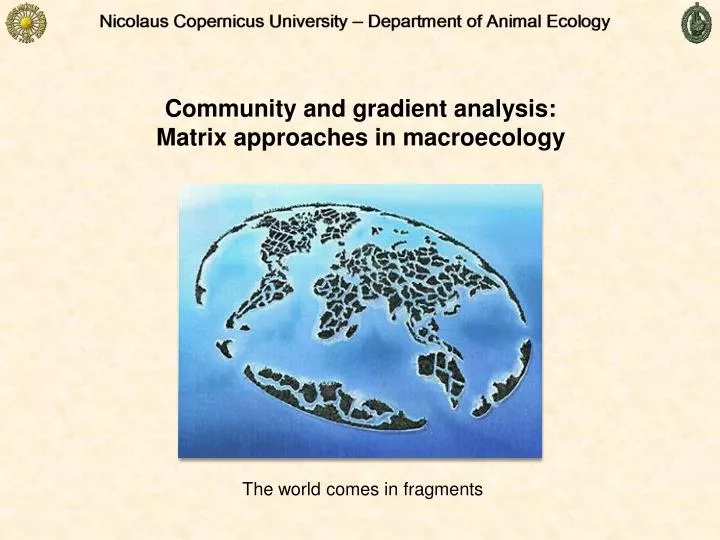
Community and gradient analysis: Matrix approaches in macroecology. The world comes in fragments. Statistical inference means to compare your hypothesis H 1 with an appropriate null hypothesis H 0 . Type I error. Type II error. But what about more complex patterns:

E N D
Community and gradient analysis: Matrix approaches in macroecology Theworldcomesinfragments
Statistical inference means to compare your hypothesis H1 with an appropriate null hypothesis H0. Type I error Type II error • But what about more complex patterns: • Relative abundance distributions • Productivity – diversity relationship • Succession • Community assembly • Simple examples in ecology are • The correlation between species richness and area (H0: no correlation, t-test) • Differences in productivity between plots of different soil properties.(H0: no difference between means, ANOVA)
We comparediversities on islands Galapagos Islands A t-testpoints to significantdifferencesindiversity. • But: Your variance estimator comes from the underlying distribution of species and individuals. • Doesthevariancestemfrom • Species interactions? • Random processes? • Evolutionary history? • Ecological history? • In fact we do not have an appropriatenullhypothesis. • Bootstrappedorjackknifedvarianceestimatorsonlycatchthevariabilityintheunderlyingdistribution.
Statisticalinference Isspeciesco-occurrence random or do specieshavesimilar habitat requirements? PF(r=0) < 0.00001 A simpleregressionanalysispoints to joint occurrences. Abundancescaleexponentially. Extremevaluesbiastheresults Spearman’sr = 0.67, PF(r=0) < 0.001 ClassicalFisheriantestingrelies on an equiprobablenullassumption. All valuesareequiprobable. In ecologythisassumptionisoften not realistic.
Species do not havethe same abundancesinthe meta-community and sitesdifferincapacity. Statisticaltestingshouldincorporatesuchdifferencesinoccurrencepobabilities. Ecologistsoftenhave a good H1hypothesis. Much discussionisabouttheappropriatenullassumption H0. What do we expectifcolonization of thesethreeislandsis random? Ecologyisinterestedinthedifferencesbetweenobservedpattern and random expectation. Ourstatisticaltestsshoulddealwiththesedifferences and not withrawpattern! If we useclassicalFisheriantestingnearlyallempiricalecologicalmatricesaresignificantly non-random. Thus we can’tseparateecologicalinteractionsfrom mass effects.
Theory of Island biogeography Galapagos Islands tries to understand diversity from a stochastic species based approach. 95% confidence limits We treat the theory as H0 We treat the theory as H1 The theory gives us random expectations. Residuals need ecological interpretation. The theory gives us expectations that have to be confirmed by observation.
Multispeciesmetapopulationand patchoccupancymodels Islands in a fragmentedlandscape Random dispersalofindividualsbetweenislandsresults in a stablepatternofcolonization The changeofoccupancy p in time depends on patch size anddistanceaccording to a logistc growth equation. Metapopulation modelsaresinglespeciesequivalentsoftheislandbiogeographymodel. Multispeciesmetapopulationmodelsgive null expectations on communitystructure.
Theneutraltheory of biodiversity • Neutral models try to explain ecological patterns by five basic stochastic processes: • Simple birth processes - Simple death processes • Immigration of individuals - Dispersal of individuals • Lineage branching Neutral models are the individual based equivalents to the species based theory of island biogeography! Although they make predictions about diversities they do not explicitly refer to species! Diversities refer to evolutionary lineages The main trigger of neutrality is dispersal. A high dispersal rates species specific traits are of minor importance for the shape of basic ecological distributions. Ecologicaldrift
Used as H1 Neutral models make explicit predictions about Shape and parameters of species rank order distributions Species – area relationships Abundance - range size relations Local diversity patterns Patterns of succession Local and regional species numbers Branching patterns of taxonomic lineages Used as H0 residuals from model predictions are measure of ecological interactions • The model contains a number of hidden variables (dispersion limitation, branching mode, dispersal probability, isolation, matrix shape… • CPU times are a limiting resource • Variable carrying capacities are needed to obtain realistic evolutionary time scales
The neutral, metapopulationandislandbiogeographymodelscontaintoomanyhidden variables tobeofuseasnull hypothesis. Ecologicalrealismwithouttoomanyparameters We neednullmodelsthatareecologicallyrealistic and rely on fewassumptionsthatapply to allspecies. Gradient of null model assumptionsincludingmore and moreconstraints. Nullmodelsonlyuseinformationgiveninthematrix. Thesesarematrixfill, marginaltotals, and degreedistributons.
Gradient of null model assumptionsincludingmore and moreconstraints. Marginaltotals Start from an emptymatric and fillitrandomlywithoutoraccording to someconstraints Degreedistribution Possibleconstraints Retainfill and rowdegreedistribution Retainrow and columntotals Retainfill Retainfill and rowtotals Retainfill and row and columndegreedistribution Retainfill and columndegreedistribution Retainfill and columntotals
Equiprobable - fixed Fixed - fixed Equiprobable - equiprobable Proportional - proportional Fixed - proportional Fixed - Equiprobable Gradient of null model assumptionsincludingmore and moreconstraints. Excludes mass effects Appropriateifnothingisknownaboutabundances and capacities Identifies most empiricalmatrices as being random Excludes most mass effects Appropriateifcolumntotalsareproportional to sitescapacities Identifies many empiricalmatrices as being random Partlyincludes mass effects Appropriateifspeciesabundancesorsitecapacitiesareequal Identifies most empiricalmatrices as being not random Partlyexcludes mass effects Appropriateifspeciesabundancesorsitecapacitiesareproportional to metapopulationabundancesorsitescapacities Identifies many empiricalmatrices as being not random Includes mass effects Most liberal Identifiesnearlyallempiricalmatrices as being not random Lowdiscriminationpower
Algorithms for thefixedfixednull model Fill algorithm An initialemptymatrixisfilled step by step at random. Ifafter a placementviolatestheaboveconstraintsitsteps back and placeselsewhere. Theprocesscontinuesuntilalloccurrencesareplaced. Major drawbacks: Long computation times Potential dead ends Swap algorithm Major drawbacks: Generatesbiasedmatricesindependence on theoriginaldistribution Thealgorithmscreenstheoriginalmatrix for checkerboards and swapsthem to leaverow and columnssumsconstant. Useatleast 10*species*sites swaps. Trial algorithm(Sum of squares reduction) Major drawbacks: Randomized matrices have a low variance that are prone to type II errors. The algorithm starts with a random matrix according to the row and column constraints and sequentially swaps all 2x2 submatrices until only 1 and 0 remain.
2000 Observed score 1500 Frequency 1000 Lower upper CL CL 500 0 3.57 3.67 3.78 3.89 3.99 4.1 Scores TheSwapalgorithmis most oftenused Sequentialswap: First make a burnin and swap 30000 times and thenuseeachfurther 5000 swaps as a new random matrix Independent swap: Generateeach random matrixfromtheoriginalmatrixusingatleast 10*species*sites swaps. Comparetheobservedmetricscoreswiththesimulatedones(100 ormorerandomizedmatrices) Z-scorelower CL = -0.37 Z-scoreupper CL = -3.00
Usingabundances Includingabundancesintonullmodelsincreasesthenumber of possiblenullmodels Populations populationsfixed proportional to observedtotals Abundance marginaltotalsfixed proportional to marginaltotals equiprobable equiprobable proportional to marginaltotals marginaltotalsfixed equiprobable Species These 27 combinationsregardrows, columns, and row and columns.
Testing of nullmodels and metricsusingproportional random matrices. Themetricsshouldn’tdetectthesematrices as being non-random. 200 random matrices
Abundancematricesaremoreoftendetected as being non-random Fraction of 185 matricesdetected as beingsignificantly (two-sided 95% CL) segregated (darkbars) oraggregated (whitebars).