Download
1 / 22
220 likes | 292 Views
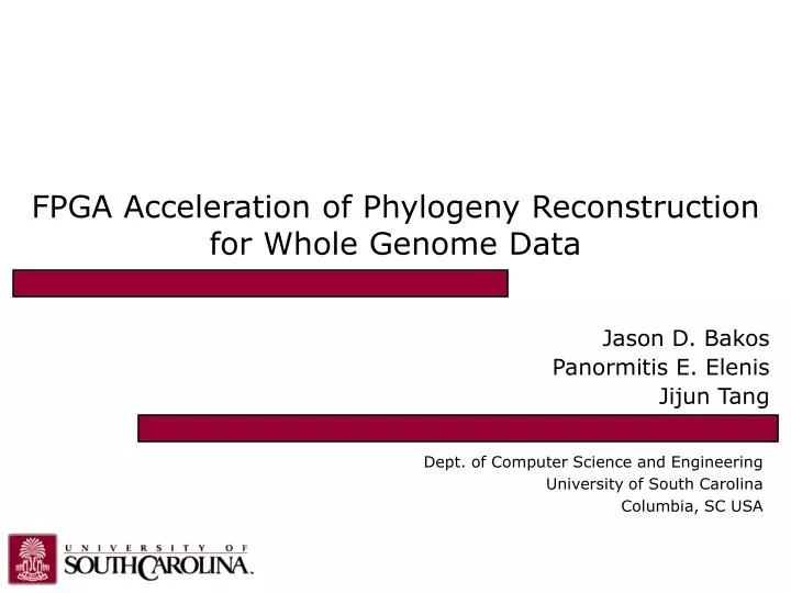
FPGA Acceleration of Phylogeny Reconstruction for Whole Genome Data. Jason D. Bakos Panormitis E. Elenis Jijun Tang. Dept. of Computer Science and Engineering University of South Carolina Columbia, SC USA. Talk Outline. FPGAs and high-performance reconfigurable computing

E N D
FPGA Acceleration of Phylogeny Reconstructionfor Whole Genome Data Jason D. Bakos Panormitis E. Elenis Jijun Tang Dept. of Computer Science and Engineering University of South Carolina Columbia, SC USA
Talk Outline • FPGAs and high-performance reconfigurable computing • Initial target application: gene rearrangement analysis • Hardware design and experimental results
High-Performance Reconfigurable Computing • HPRC: • Use FPGA as co-processor • Example: • Application requires a week of CPU time • One computation consumes 99% of execution time • Replaces software • Exploits parallelism
HPRC: Requirements, Pros, Cons • Application criteria: • computationally expensive • has a bottleneck computation • bottleneck computation is parallelizable • …and has low I/O and storage requirements • Advantages of HPRC: • Cost • FPGA card => ~ $15K • 128-processor cluster => ~ $150K + maintenance + cooling + electricity + recycling • Disadvantage for HPRC: • Programming the FPGA
Programming an FPGA • Requires large-scale digital logic design • Instance and interconnect logic and memories • Especially difficult for control-dependent computations • Even worse… • To achieve performance: • Finely parallelize algorithm across FPGA resources • Our solution: • Develop a pre-designed library of kernels for computational biology • Develop a design toolthat uses this library to generate accelerators
Talk Outline • FPGAs and high-performance reconfigurable computing • Initial target application: gene rearrangement analysis • Hardware design and experimental results
Target Application • Gene rearrangement analysis • Evolution analysis using gene order data • Assumes gene-rearrangement model for evolution, i.e.: • Inversion g0 g1g2 g3 g4 g5g0 g1–g4 –g3 –g2 g5 • Transposition g0 g1g2 g3 g4 g5 g0g2 g3 g4 g1 g5 • Transversion g0 g1g2 g3 g4 g5 g0–g4 –g3 –g2 g1 g5
Reconstruction Method • Maximum parsimony: • Search for tree with minimum number of rearrangement events • Direct-optimization method: • To evaluate a fixed tree… • Label all internal vertices with gene orders • Initialize and iteratively refine until the labels converges • Measure edge lengths using distance estimator … … , ,
M A B C Median • Median computation used to label internal vertices • Find M that minimizes d(A,M) + d(B,M) + d(C,M) for some distance measure d() • For gene rearrangement data: • Optimal solution is NP-hard in “diameter” of inputs: d(A,B) + d(A,C) + d(B,C) d(A,M) d(B,M) d(C,M)
Execution Behavior • Application behavior depends on evolution rate of inputs • Execution time ratio for median computations: • Asymptotically approaches 100% with diameter of input set • Median adopted as kernel computation 1 Execution Time Ratio for Labeling 0 Evolution Rate of Inputs
Breakpoint Median • Construct a fully connected graph containing all gand –g for each gene • w(g,-g) = -¥ • Initialize all other weights to be 3 • For each adjacency gh in the three genomes, decrement weight between vertex –g and h • Solve TSP - - + + 1 2 1 2 A = -1 +2 -4 -3 B = -1 -2 +3 +4 C = -2 +3 +4 +1 cost = -¥ cost = 0 cost = 1 cost = 2 - + - + + - + - 4 3 4 3 - + - + An optimal solution corresponding to genome +1 +2 -3 -4 Edges not shown have cost = 3
Breakpoint Median Algorithm • Optimal solution is feasible due to small graph • Algorithm: • Represent TSP graph as a list of edges • Test every possible valid combination of edges • Implemented as a branch-and-bound search • Upper bound is the best tour found so far • Lower bound is computed using a greedy algorithm • Loop that inspects each vertex in TSP graph • Accumulates lower bound value (based on search state) • Performed each time an edge is added or deleted from solution state • Requires nearly 100% of median execution time (bottleneck)
pruned Example Breakpoint Median sorted edge list: (-3,4,w=0) (2,3,w=1) (1,2,w=2) (-1,-2,w=2) (1,-2,w=2) (-2,-4,w=2) (-1,3,w=2) (-1,-4,w=2) (1,-4,w=2) used 1 => 0 -1 => 0 2 => 0 -2 => 0 3 => 0 -3 => 0 4 => 0 -4 => 0 otherEnd 1 => -1 -1 => 1 2 => -2 -2 => 2 3 => -3 -3 => 3 4 => -4 -4 => 4 1 -1 2 -2 3 -3 4 -4 cost = 0 used 1 => 0 -1 => 0 2 => 0 -2 => 0 3 => 0 -3 => 1 4 => 1 -4 => 0 otherEnd 1 => -1 -1 => 1 2 => -2 -2 => 2 3 => -4 -3 => 3 4 => -4 -4 => 3 1 -1 2 -2 3 -3 4 -4 used 1 => 0 -1 => 0 2 => 1 -2 => 0 3 => 1 -3 => 1 4 => 1 -4 => 0 otherEnd 1 => -1 -1 => 1 2 => -2 -2 => -4 3 => -4 -3 => 3 4 => -4 -4 => -2 cost = 0 1 -1 2 -2 3 -3 4 -4 cost = 1
Example Breakpoint Median sorted edge list: (-3,4,w=0) (2,3,w=1) (1,2,w=2) (-1,-2,w=2) (1,-2,w=2) (-2,-4,w=2) (-1,3,w=2) (-1,-4,w=2) (1,-4,w=2) used 1 => 0 -1 => 0 2 => 0 -2 => 0 3 => 0 -3 => 0 4 => 0 -4 => 0 otherEnd 1 => -1 -1 => 1 2 => -2 -2 => 2 3 => -3 -3 => 3 4 => -4 -4 => 4 1 -1 2 -2 3 -3 4 -4 cost = 0 used 1 => 0 -1 => 0 2 => 0 -2 => 0 3 => 0 -3 => 1 4 => 1 -4 => 0 otherEnd 1 => -1 -1 => 1 2 => -2 -2 => 2 3 => -4 -3 => 3 4 => -4 -4 => 3 used 1 => 1 -1 => 0 2 => 1 -2 => 0 3 => 0 -3 => 1 4 => 1 -4 => 0 otherEnd 1 => -1 -1 => -2 2 => -2 -2 => -1 3 => -4 -3 => 3 4 => -4 -4 => 3 1 -1 2 -2 3 -3 4 -4 exclude edge (2,3) 1 -1 2 -2 3 -3 4 -4 cost = 0 cost = 2 used 1 => 1 -1 => 1 2 => 1 -2 => 1 3 => 1 -3 => 1 4 => 1 -4 => 1 otherEnd 1 => -1 -1 => 3 2 => -2 -2 => -1 3 => -1 -3 => 3 4 => -4 -4 => 3 used 1 => 1 -1 => 0 2 => 1 -2 => 1 3 => 0 -3 => 1 4 => 1 -4 => 1 otherEnd 1 => -1 -1 => 3 2 => -2 -2 => -1 3 => -1 -3 => 3 4 => -4 -4 => 3 1 -1 2 -2 3 -3 4 -4 1 -1 2 -2 3 -3 4 -4 cost = 6 cost = 4 tour is -1, 1, 2, -2, -4, 4, -3, 3 median is -1, 2, -4, -3
Talk Outline • FPGAs and high-performance reconfigurable computing • Initial target application: gene rearrangement analysis • Hardware design and experimental results
Hardware Median Core Design Top-Level Controller
Parallelizing the Median Computation • Exploit both fine- and coarse- grain parallelism • Fine-grain • Unroll loop for lower bound computation • Perform multiple iterations in parallel • Coarse-grain • Use parallel median cores for single median computation • Partition search space
Fine-Grain Parallelism Lower bound unit: used table v=2 e0=11 e1=-19 e2=-49 used(v) used(e0) used(e1) used(e2) if used(v) = 0 then VALID_WEIGHTS= f for i = 0 to edge_count(v) - 1 if used(ei) = 0 and otherEnd(v) != ei and excludedi(v) != 1 then add weighti to VALID_WEIGHTS end if end loop if VALID_WEIGHTS is empty lower_bound = lower_bound + 3 else lower_bound = min(VALID_WEIGHTS) end if TSP graph representation: 1 (1,-4),w=0 -1 (-1,9),w=1 (-1,25),w=2 2 (2,11),w=2 (2,-19),w=2 (2,-49),w=2 -2 (-2,17),w=2 (-2,20),w=1 . . . -19 (-19,2),w=2 (-19,-4),w=2 (-19,10),w=2 . . . otherEnd table otherEnd(v) v=2 excluded table excluded0(v) excluded1(v) excluded2(v) v=2 edge_count table 3 v=2 11 -19 weight0 weight1 weight2 2 2 2 2 2 2 2 -49
Coarse-Grain Parallelism • Parallelize search => partition TSP search space • Problems: • High amount of state information (communication overhead) • Dynamic load balancing would be complex (control overhead) • Solution: “virtually” partition the TSP search space • Search order determined by ordering of edge list • Use parallel median cores • Each core uses unique search order • All cores share a global upper bound value
Experimental Results: Median Acceleration • Best performance was achieved: • 20 lower bound units per core • 2 cores • ~ 50% of FPGA resources • Performance improves with size of search space • i.e. search time • Host-FPGA communication overhead Average speedup for 1000 median computations
Experimental Results: Application Acceleration • Perform end-to-end reconstruction procedure • Dispatch all median computations to FPGA Average speedup for 10 end-to-end reconstructions
Conclusions and Future Work • Achieved 100X end-to-end application speedup for distantly related data sets • Demonstrated that FPGAs can accelerate this class of application • Future Work: • Additional kernel designs (i.e. tree generation) • Implement heterogeneous mix of kernels on the FPGA according to evolution rate of input set