Download
1 / 9
90 likes | 179 Views
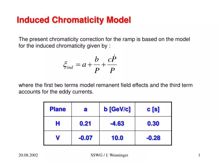
Induced Chromaticity Model. The present chromaticity correction for the ramp is based on the model for the induced chromaticity given by : where the first two terms model remanent field effects and the third term accounts for the eddy currents. Chromaticity trims in the ramp.

E N D
Induced Chromaticity Model The present chromaticity correction for the ramp is based on the model for the induced chromaticity given by : where the first two terms model remanent field effects and the third term accounts for the eddy currents. SSWG / J. Wenninger
Chromaticity trims in the ramp • The model does not fully account for the observed chromaticity : • important trims are required in addition. • less efficient cycle setups. • trims are copied from one cycle to the next (and not always in the best way..). Goal of this analysis : • Recover the trims under known conditions (i.e. with complete chromaticity measurements [multiQ]) : • 2 nominal LHC cycles (537,540) to 540 GeV. • one special LHC cycle (542) to 80 GeV. • Check the reproducibility. • Establish a better model. • … SSWG / J. Wenninger
LHC Ramp Chromaticity Trims • Reconstructed total trim to obtain x ~ +0.05 to +0.1 in the ramp (2 cycles). • Trims are reconstructed from the PC currents (“bug” in the target function setting). • Reproducibility is good, ~ 0.05 or better. Correction of the natural chromaticity (x ~ 1.26) excluded ! SSWG / J. Wenninger
Model versus Trims Example of the difference between total trim[] and modeled trim [-]. Observed Dx ~ twice as large as model. Un-modeled “bump” peaking @ 400 GeV. SSWG / J. Wenninger
Model versus Trims (II) Difference between total trim[] and modeled trim [-] – 80 GeV cycle. Change due to dP/dt (eddy currents) ~ correct ! Measured x is smooth over this transition. SSWG / J. Wenninger
Model Improvement • The default model cannot account for the “bump” between 100 and 400 GeV… • Empirically add a term : • where p0 ~ 400 GeV/c. Very good fit, but with different values for a and b. The eddy current term c ~ unchanged. SSWG / J. Wenninger
b3 Components in Dipoles With Angeles Faus-Golfe’s SPS model including field errors (b3, b4, b5), one can convert the chromaticity trims into b3 field components for the MBA and MBB dipoles. The relation between chromaticity and b3 components is : (b3 in 10-3 m-2), Q’ is the “usual” chromaticity…. SSWG / J. Wenninger
b3 Components in Dipoles (II) Uncertainties on b3 ~ 0.4 10-3 m-2 Results from measurements @ 26 GeV in 2001 SSWG / J. Wenninger
Summary • For the LHC cycles in the SPS : • the chromaticity trims seem to be very reproducible, but we must be careful when copying trims between cycles. • the present model for the chromaticity is off by a factor ~ 2, it can be improved by an empirical correction. • Next step : • During the next long MD, trim back the settings of the FT cycle to the time of the setup where x was measured over most of the cycle. Recover the sextupole currents and reconstruct the trims. • Refit the model with the FT settings, consistency with LHC cycle. • For FT, the eddy currents effects are much more violent. SSWG / J. Wenninger