Download
1 / 23
230 likes | 611 Views
Models of Volatility Smiles II. Chapter 9: ADVANCED OPTION PRICING MODEL. Three Alternatives to Geometric Brownian Motion. Stochastic Volatility by Heston (1993) Implied Volatility Function Model by Andersen and Brotherton-Ratcliffe (1997/98)

E N D
Models of Volatility Smiles II Chapter 9: ADVANCED OPTION PRICING MODEL
Three Alternatives to Geometric Brownian Motion • Stochastic Volatility by Heston (1993) • Implied Volatility Function Model by Andersen and Brotherton-Ratcliffe (1997/98) • Jumps and Stochastic Volatility Model by Duffie, Pan and Singleton (2000)
Time Varying Volatility • Suppose the volatility is s1 for the first year and s2 for the second and third • Total accumulated variance at the end of three years is s12 + 2s22 • The 3-year average volatility is
Stochastic Volatility Models • When V and S are uncorrelated a European option price is the Black-Scholes price c integrated over the distribution of the average variance g is the probability density function of in a risk-neutral world.
Stochastic Volatility Models (Cont’d) • When V and S are negatively correlated we obtain a downward sloping volatility skew similar to that observed in the market for equities • When V and S are positively correlated the skew is upward sloping
Heston Model • The popular Heston model is a commonly used SV model, in which the randomness of the variance process varies as the square root of variance. In this case, the differential equation for variance takes the form: where is the mean long-term volatility, is the rate at which the volatility reverts toward its long-term mean, is the volatility of the volatility process, and dBt is, like dWt, a Gaussian with zero mean and unit standard deviation. However, dWt and dBt are correlated with the constant correlation value . The model has CIR dynamics.
Heston Model • In other words, the Heston SV model assumes that volatility is a random process that 1. exhibits a tendency to revert towards a long-term mean volatility at a rate , 2. exhibits its own (constant) volatility, , 3. and whose source of randomness is correlated (with correlation ) with the randomness of the underlying price processes. • 5 time-homogeneous parameters {v0,,,,}. Will not go to zero if 2>2 • Psuedo-analytic pricing of Europeans
Partial Differential Equation • Value function of a general contingent claim g(S)=U(T,v,S) with boundary conditions
Heston Characteristic Function • Pricing European options • Fourier inversion Im(.): imaginary part • Characteristic function form
Heston Model • Substitute the proposed solution into previous PDE and define x=lnS, Heston obtains for j=1,2
SV European Options • With characteristic function where Re(.): real part
The Implied Volatility Models • Two models both match the risk-neutral probability distribution: the implied volatility function (IVF) model by Dupire (1994) and Andersen and Brotherton-Ratcliffe (1997/98) and the implied tree model by Rubinstein (1994)
The IVF Model • The implied volatility function model is designed to create a process for the asset price that exactly matches observed option prices. The usual geometric Brownian motion model is replaced by
The Volatility Function(Andersen and Brotherton-Ratcliffe) 1997/98 • The volatility function that leads to the model matching all European option prices is • If a sufficiently large number of European call prices are available in the market, this equation is used to estimate (S,t) function with some smoothing of the observed volatility surface. • The option prices can be priced by plugging this local volatility function (S,t) into a numerical methods (Monte-Carlo, trinomial tree or most efficiently a PDE).
Strengths and Weaknesses of the IVF Model • The model matches the risk-neutral probability distribution of stock prices assumed by the market at each future time. Therefore, options providing payoffs at just one time are priced correctly. • The models does not necessarily get the joint probability distribution of stock prices at two or more times correct. Therefore, exotic options such as compound options and barrier options may be priced incorrectly.
Stochastic Volatility Model with Jumps • Duffie, Pan and Singleton (2000) provide a European option formula for the stochastic volatility model with jumps based on transform analysis. The model consists of two correlated stochastic processes between the log of stock prices Y=lnS and the volatility v where are constants. Z: Poisson jump; WQ: Random vector for the diffusion processes of log of price and volatility v.
Partial Differential Equation • The jumps are with an arrival intensity and normally distributed jump size with mean and variance The partial differential equation of the risk-neutral process for the early-exercise premium in the continuation region is where expected jump rate is
SV and Jumps European Options • Options: where
Example • Where
Example (Cont’d) • Also, where
Example (Cont’d) • Jumps in Y, arrival intensity y, normally distributed jump size, mean y and variance • Jumps in v, arrival intensity v, exponentially jump size, mean v • Simultaneous correlated jumps in Y and v, arrival intensity c, marginal distribution of jump size in v with exponential mean c,v • Jumps in Y conditional on jump size in v,zv, normally distributed with mean c,y+Jzv and variance
Empirical Review • Bakshi, Cao and Chen (1997) and Bates (1997), SVJ-Y: The model allows negative jumps in Y and increases the skewness of the distribution of YT, does not generate the level of skewness implied by the volatility smirk in market data. They suggest double jumps for better fitting to market data.
Model Selection • SV: Stochastic volatility model with no jumps, • SVJ-Y: Stochastic volatility model with jumps in price only, • SVJJ: Stochastic volatility with simultaneous and correlated jumps in price and volatility,