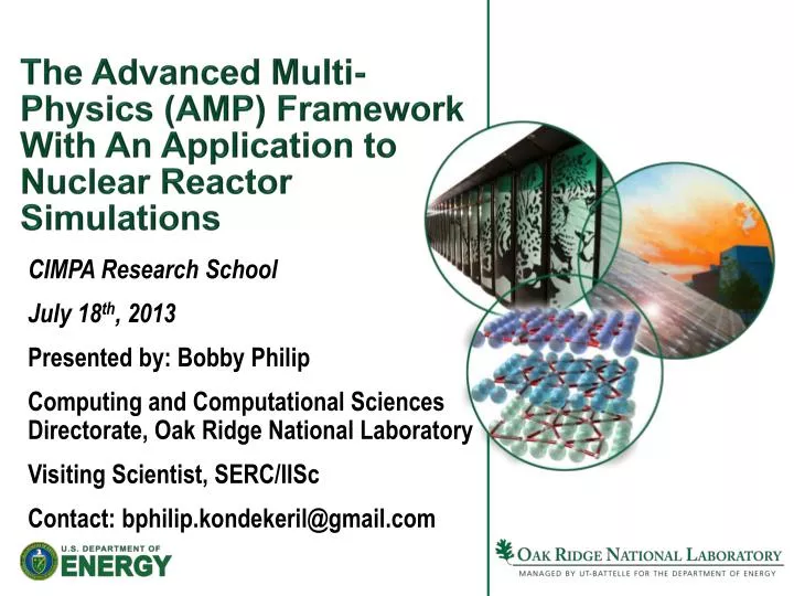
The Advanced Multi-Physics (AMP) Framework With An Application to Nuclear Reactor Simulations

1. The Advanced Multi-Physics (AMP) Framework With An Application to Nuclear Reactor Simulations CIMPA Research School July 18th, 2013 Presented by: Bobby Philip Computing and Computational Sciences Directorate, Oak Ridge National Laboratory Visiting Scientist, SERC/IISc Contact: bphilip.kondekeril@gmail.com

2. Funding and Contributors: • Funding: • HPC Liaison Activities: National Center for Computational Science (NCCS), Oak Ridge National Laboratory (ORNL) • AMP: Nuclear Energy Advanced Modeling and Simulation (NEAMS) program of the U.S. DOE Office of Nuclear Energy • Contributors: • Jack Wells (NCCS Director of Science), B. Messer (NCCS Scientific Computing Group Leader), NCCS Users • AMP: • K. Clarno, R. Sampath, M. Berrill,, S. Hamilton, S. Allu, J. Banfield, A. Philippe, • Alumni: W. Cochran, G. Dilts, , G. Yesilyurt, P. BaraiJ. Lee, P. Nukala, B. Mihaila

3. Outline • An Introduction to ORNL and the Oak Ridge Leadership Computing Facility • Description of the Advanced Multi-Physics Framework (AMP) • Modeling Nuclear Reactor Assemblies With AMP

4. Deliver scientific discoveries and technical breakthroughs that will accelerate the development and deployment of solutions in clean energy and global security, and in doing so create economic opportunity for the U.S. ORNL’s mission 4 Managed by UT-Battelle for the U.S. Department of Energy

5. Science Strategy for the Future:Major Laboratory Initiatives Enhance building energy efficiency, sustainable transportation, and advanced manufacturing Deliver science using neutrons Scale computing, data infrastructure, and analytics for science Discover and demonstrate advanced materials for energy Advance scientific basis for new nuclear technologies and systems Advance understanding in biological, environmental systems, and climate change impacts science Solve the nation’s most compelling global security challenges

6. What is the Leadership Computing Facility? • Collaborative, multi-lab, DOE/SC initiative ranked top domestic priority in Facilities for the Future of Science: A Twenty-Year Outlook. • Mission: Provide the computational and data science resources required to solve the most important scientific & engineering problems in the world. • Highly competitive user allocation program (INCITE, ALCC). • Projects receive 100x more hours than at other generally available centers. • LCF centers partner with users to enable science & engineering breakthroughs(Liaisons, Catalysts).

7. ORNL’s “Titan” Hybrid System: World’s Most Powerful Computer #1 • SYSTEM SPECIFICATIONS: • Peak performance of 27.1 PF • 24.5 GPU + 2.6 CPU • 18,688 Compute Nodes each with: • 16-Core AMDOpteron CPU • NVIDIA Tesla “K20x” GPU • 32 + 6 GB memory • 512 Service and I/O nodes • 200 Cabinets • 710 TB total system memory • Cray Gemini 3D Torus Interconnect • 8.9 MW peak power 4,352 ft2 404 m2

8. High-impact science at OLCF across a broad range of disciplines. For example in 2012: Materials: Quantum Magnets “Bose glass and Mott glass of quasiparticlesin a doped quantum magnet” Rong Yu (Rice U.) Nature (2012) Nuclear Physics “The Limits of the Nuclear Landscape” J. Erier, (UT/ORNL) Nature (2012) CoolingStableWarming Carbon Nanomaterials “Covalently bonded three-dimensional carbon nanotube solids via boron induced nanojunctions” Hashim (Rice), Scientific Reports (2012) Climate Prediction and Mitigation “Relative outcomes of climate change mitigation related to global temperature versus sea-level rise” G.A. Meehl (NCAR), Nature Climate Change (2012) Insert graphic here Paleoclimate Climate Change “Global warming preceded by increasing carbon dioxideconcentrations during the last deglaciation” J. Shakun, (Harvard/Columbia) Nature (2012) Plasma Physics: “Dynamics of relativistic transparency and optical shuttering in expanding overdense plasmas” S. Palaniyappan(LANL) Nature Physics (2012)

9. Science challenges for LCF in next decade Combustion Science Increase efficiency by 25%-50% and lower emissions from internal combustion engines using advanced fuels and new, low-temperature combustion concepts. Climate Change Science Understand the dynamic ecological and chemical evolution of the climate system with uncertainty quantification of impacts on regional and decadal scales. Biomass to Biofuels Enhance the understanding and production of biofuels for transportation and other bio-products from biomass. Fusion Energy/ITER Develop predictive understanding of plasma properties, dynamics, and interactions with surrounding materials. Globally Optimized Accelerator Designs Optimize designs as the next generations of accelerators are planned, increasingly detailed models will be needed to provide a proof of principle and a cost-effective method to design new light sources. Solar Energy Improve photovoltaic efficiency and lower cost for organic and inorganic materials.

10. DOE Computational Facilities Allocation Policy for Leadership Facilities Primary Objective: • “Provide substantial allocations to the open science community through a peered process for a small number of high-impact scientific research projects” 10% Director’s Discretionary 60% INCITE 30% DOE “ASCR Leadership Computing Challenge”

11. OLCF allocation programsSelecting applications of national importance 60% 30% 10% Director’s Discretionary

12. 2014 INCITE Call for Proposals • Planning Request for Information (RFI) • Call opens April, 2013. Closes June, 2013 • Expect to allocate more than 5 billion core-hours • Expect 3X oversubscription • Awards to be announced in November for CY 2014 • Average award to exceed 50 million core-hours Number of 2013 INCITE Submittals by PI Affiliation Reaching out to Researchers Contact information Julia C. White, INCITE Manager whitejc@DOEleadershipcomputing.org Nearly 50% of the non-renewal proposals are by new PIs.

13. The Advanced Multi-Physics Package: Design and Capabilities

14. Design Objectives • Provide a complete object-oriented simulation system for time-dependent and steady state multi-scale multi-domain coupled physics • Enable algorithmic research through extensible design: • Single and Multiple Domain Meshing • Load Balancing • Linear Algebra • Discretizations • Multi-Physics Couplings • Multi-Scale Couplings • Solution Transfer • Linear and Nonlinear Solution Methods • Time Integration • Intrusive and non-intrusive UQ • Data Assimilation

15. Design Objectives • Maximize use of existing high quality scientific computing software through standard interfaces: PETSc, Trilinos, SUNDIALS, Dakota, Denovo, STKMesh, MOAB • Enable incremental development in simulation of multi-physics systems without forced code rewrite as new physics introduced • Enable code-reuse for legacy applications • Ensure long term stability and viability by loose coupling to external packages

16. Mesh libMesh AMP::Mesh stk::mesh User::Mesh • Common Mesh Interface • Standard set of function provided including: • Number of local and global elements, iterators, • Mesh identification/names, subsets, etc. • Provides wrapper to underlying mesh packages • libmesh and stk::mesh currently implemented • MOABin progress • User defined mesh packages are possible Mesh M1 M2 M3 M4 MultiMesh SubsetMesh Local / Global Size Communicator • MultiMesh • Multiple meshes may be combined into a multi-mesh • MultiMesh is just another mesh with full functionality Set/Get Mesh Name Get MeshID • SubsetMesh • Any mesh can be subset to produce a subset-mesh • SubsetMesh is just another mesh with full functionality Mesh Iterators Displace Mesh Subset

17. Mesh Multiple Domain / Multiple Processor decomposition Shown: 3 domains, each with different processor decomposition. The color indicate the ranks of the owning processor Easy subsetting to create new mesh domains Shown: A sample subset over the previous mesh (left) for a surface. The color represents an arbitrary vector over the domain.

18. Linear Algebra PETSc Vector Epetra Vector Sundials Vector Simple Vector Vectors • AMP provides a common Vector / Matrix interface • Ghost communication is handled in AMP • All basic Linear Algebra function provided V1 V2 V3 MultiVector • Underlying vector data may come from different • places: Epetra, PETSc, SUNDIALS, std::vector, etc. Views • MultiVectorcapabilities • MultiVector can compose multiple vectors of different types • All the same vector functions extend to MultiVector • Subset vectors for particular variables, stride, mesh, etc. Managed PETSc Vector Managed Epetra Vector • Views to different vectors • Allows one package to see data from another as if it were its own • Example: PETSc will use a view of a EpetraVector Managed Sundials Vector Subset Vector

19. Linear Algebra MultiMesh/MultiPhysics M1 M3 M2 Single Vector MultiVector V1 V2 V3 Single Matrix Single Matrix Multiblock Matrix M11 M12 M13 M21 M22 M23 M31 M32 M33

20. Operators Domain Range • Operations: • apply(): action of operator on vector • getJacobianParameters(): parameters for linear approximation • reset(): reset or re-initialize an operator

21. Operator Example apply(T, r) NonlinearDiffusionOperator getJacobianParameters(T0) reset(params)

22. Operators: Local Physics Models • Implements constitutive law at local element level – eg diffusion coefficient, material models (mechanics) • Not a requirement but considerably increases code re-use

23. Operators: Boundary • Can have local physics model • Defined on boundary subdomain • Composed to obtain complex boundary operators • Same interface as other operators with • Dirichlet, Neumann, Robin FEM Boundary Operators provided Robin BoundaryOp Neumann BoundaryOp Conductivity Local Model Conductivity LocalModel Composite Boundary Operator

24. Operators: BVPOperator • A VolumeOperator and a BoundaryOperator together can form a BVPOperator • Convenient for solving boundary value problems BVPOperator apply() VolumeOperator getJacobianParameters() BoundaryOperator reset()

25. Operators: MapOperator • Transfer data between domains • Projection operators between spaces BVPOperator BoundaryOperator MapOperator BoundaryOperator BVPOperator

26. Operator: ColumnOperator • Each operator can itself be composed of multiple operators • This is how we rapidly build multi-physics operators and/or multi-domain operators • Operator interface remains the same Multi-domain Thermal Operator Multi-domain Thermal Operator Multi-domain Mechanics Operator Multi-domain Mechanics Operator Thermal Operator Thermal Operator Mechanics Operator Mechanics Operator Thermal Operator Thermal Operator Mechanics Operator Mechanics Operator Multi-Domain Thermal Operator ThermalOp ThermalOp ThermalOp ThermalOp ThermalOp Thermal Operator Thermal Operator Mechanics Operator Mechanics Operator Multi-Domain Thermo-Mechanics Operator Mech. Op Mech. Op Mech. Op Mech. Op Mech. Op Thermal Operator Thermal Operator Mechanics Operator Mechanics Operator Multi-Domain Mechanics Operator Multi-domain Thermal Operator Multi-domain Thermal Operator Multi-domain Thermal Operator Multi-domain Thermal Operator Multi-domain Thermal Operator Multi-domain Thermal Operator Multi-domain Multi-Physics Operator Multi-domain Multi-Physics Operator Multi-domain Multi-Physics Operator

27. Operators: Discretization • Operators with different discretizations can be created • AMP currently provides a library of FEM Operators • FEM assembly is not user responsibility • User only needs to supply local physics model • User can create new FEM Operators that leverage existing capabilities • Can couple operators discretized with different spatial dimensions, discretizations, e.g. multi-continua

28. Operators: Summary • Operators derived from Operator base class • Provide implementations for apply(), getJacobianParameters(), reset() • Linear, Nonlinear, Time dependent, Composite System PDE, and BoundaryOperators available • FEM operators available • Nonlinear and linear diffusion • Nonlinear and linear mechanics • Nonlinear and linear Dirichlet, Neumann, Robin boundary • User free to add multi-physics of choice through operators

29. Material Database Interface • Standard interface to material properties • Used for local constitutive laws • Oft-neglected aspect within standard packages • Very important to application scientists • Material interface designed for the possibility of spawning subscale calculations for material properties

30. Solvers Domain Range • Operations • registerOperator() • solve() • reset() • resetOperator() • registerOperator(): register forward operator • solve(): compute approximate inverse • reset(): reset solver parameters • resetOperator(): reset forward operator

31. Solvers • Nonlinear solvers, linear solvers, and preconditioners all have same interface • Solvers can be composed and/or nested to create more complex solvers; multi-physics multi-domain solvers are constructed this way NonlinearSolver LinearSolver Preconditioner Multi-Domain Preconditioner Single Domain Preconditioner PC 1 PC 2 PC 3 PC .. PC n

32. Solvers • Freedom to compose solvers allows us to develop fully coupled and operator split solvers and experiment with both • AMP provides implementations of inexact Newton (PETSc, Trilinos), Nonlinear Accelerated Krylov, Krylov solvers (PETSc), multigrid (Trilinos), block diagonal preconditioners (AMP::ColumnSolver) • User is free to create new solvers that can be used with other AMP Operators and TimeIntegrators

33. Time Integrators • All time integrators derived from TimeIntegrator base class • Explicit, Implicit, Semi-implicit possible • Several concrete explicit time integrators working with FV operators: RK2, RK3, RK23 • Implicit BE and BDF2-5 integrators available through SUNDIALS interface • A time integrator can itself call other time integrators for implementing semi-implicit schemes • Time integrators use existing spatial operators, no code rewrite necessary to go from stationary to time dependent problem

34. External Software and AMP Availability • PETSc: Native and managed PETSc vectors and matrices, Krylov solver and SNES solver interfaces • Trilinos: STKMesh Mesh Management interfaces, native Epetra vector and matrix interfaces, Thyra vector interfaces, ML (Multigrid) Solver interface, NOX (inexact Newton) Solver • SUNDIALS: Native and managed SUNDIALS vector interfaces, IDA time integrator interfaces • LibMesh: Mesh interface, FEM discretization interface • HDF5, Silo, MPI, MOAB AMP Availability: open source software with modified BSD license, available on request. Please contact philipb@ornl.gov or talk to me.

35. Nuclear Fuel Assembly Simulations With AMP

36. Mechanical Response Heat Generation Secondary Systems Chemistry Heat Transport ESBWR Reactor Simulation Requires Modeling Many Coupled Physics at Many Scales 12 orders of magnitude in time 5 orders of magnitude in space

37. Radial Slice Single Lattice 20 cm 8 meters Reactor Core ESBWR The Physical Space is Large Reactor Vessel 15 meters 5 mm Single Pincell

38. Fission Distributions ~360 pellets within a 12’ fuel pin Single pellet 2cm high 2D view of distribution within assembly Collapsed view of assembly power 264 fuel pins within a 12’ assembly 4

39. Neutronics Source-Term Material variation with time (burnup) • Neutrons collide with uranium, which fissions • Heat is generated (thermal source) • New isotopes are created • Material swells (volumetric strain) • Material properties change • Additional neutrons are produced, which sustains the reaction 4

40. Thermal Model: Pellets

41. Thermal Model: Clad

42. Thermal properties

43. Mechanics • The balance of momentum: • : Cauchy stress tensor • : body force vector • : displacement vector • : density • Quasi-static assumption, inertia can be neglected: • Strain-displacement relation: • Stress-strain relation: • Small strain assumption: • VonMiseselasto-plastic model for • Thermal strain:

44. Mechanics • Bottom Pellet and Clad: (i=1) • Other Pellets: (i=2,..,N)

45. Modeling Approximations and Discretization • Modeling Approximations: • Axi-symmetric heat flux from pellets • Thermal equations currently do not depend on displacements • Gap size between pellets and clad has a significant effect on heat flux • Fission gas effects neglected • No contact between pellets and clad • Pellets are currently ‘tied’ at boundaries for mechanics • Discretization: Linear FEM discretization for thermal and mechanics

46. Solution Methodology • Discretization leads to a system of equations: • A variety of solution methods can be used to solve the above nonlinear system: • Picard • Newton • Nonlinear Gauss-Seidel • Nonlinear Krylov • Within AMP any of these solution methods is possible with potentially minimal changes

47. Classical Newton • Classical Newton • Hence, the k-th step involves inverting • q-quadratic convergence with a good initial guess:

48. Inexact Newton • With inexact Newton methods, is not inverted exactly. • Instead, we only require • Such methods give q-linear convergence. • Iterative methods can be used for approximate inversion at each Newton step.

49. Jacobian-Free Newton Krylov (JFNK) Methods • Krylov methods (GMRES in particular), are used to invert at each Newton step. • GMRES only requires the user to provide the Jacobian-vector products, • These can be approximated by • The resulting method is called a Jacobian-free Newton-Krylov (JFNK) method. • Function evaluation and preconditioning setup/apply are the only user provided operations.

50. Preconditioning • Right-preconditioning of the Newton equations is used, i.e., we solve • For Krylov methods this requires the Jacobian-vector products: • The approximate Jacobian-vector is computed in two steps: