Download
1 / 11
120 likes | 143 Views
Data Preprocessing: An Overview Data Quality Major Tasks in Data Preprocessing Data Cleaning Data Integration Data Reduction Data Transformation and Data Discretization Summary. Chapter 3: Data Preprocessing. 1. Data Integration. Data integration :

E N D
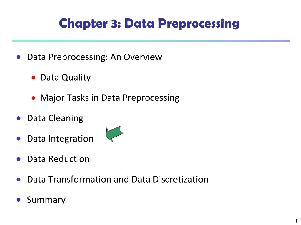
Data Preprocessing: An Overview Data Quality Major Tasks in Data Preprocessing Data Cleaning Data Integration Data Reduction Data Transformation and Data Discretization Summary Chapter 3: Data Preprocessing 1
Data Integration • Data integration: • Combines data from multiple sources into a coherent store • Careful integration can help reduce and avoid redundancies and inconsistencies • Entity identification problem: How can equivalent real-world entities from multiple data sources be matched up? • Identify real world entities from multiple data sources, Schema integration e.g., A.cust-id B.cust-# . • Detecting and resolving data value conflicts • For the same real world entity, attribute values from different sources are different • Possible reasons: different representations, different scales, e.g., metric vs. British units 2
Handling Redundancy in Data Integration • Redundant data occur often when integration of multiple databases • Object identification: The same attribute or object may have different names in different databases • Derivable data: One attribute may be a “derived” attribute in another table, e.g., annual revenue • Redundant attributes may be able to be detected by correlation analysis and covariance analysis • Careful integration of the data from multiple sources may help reduce/avoid redundancies and inconsistencies and improve mining speed and quality 3
Correlation Analysis (Nominal Data) • Χ2 (chi-square) test • The larger the Χ2 value, the more likely the variables are related • The cells that contribute the most to the Χ2 value are those whose actual count is very different from the expected count • Correlation does not imply causality • # of hospitals and # of car-theft in a city are correlated • Both are causally linked to the third variable: population
Correlation Analysis (Nominal Data) • To calculate the expected value use formula: • where n is the number of data tuples, count(A = ai) is the number of tupls having value ai for A, and count(B = bj) is the number of tupls having value bj for B . • The χ2 statistic tests the hypothesis that A and B are independent, that is, there is no correlation between them. Data Mining: Concepts and Techniques
To judge there are correlation between A and B ,we should find the χ2 static from the static table based on degree of freedom df= (r-1)*(c-1) , where r rows and c columns and choose α value . • If χ2 statistic less than or equal the χ2 calculated value , then there are strong correlation between two attributes . Data Mining: Concepts and Techniques
Chi-Square Calculation: An Example • Χ2 (chi-square) calculation (numbers in parenthesis are expected counts calculated based on the data distribution in the two categories) • expected = count (male)*count(fiction)/N = 300 * 450 / 1500 =90
Chi-Square Calculation: An Example • For this 2 × 2 table, the degrees of freedom are (2 − 1)(2 − 1) = 1. For 1 degree of freedom. • Let’s chose α=.005 , the χ2 statistic = 10.597 • χ2 statistic (chi-square) <Χ2 calculated , • 10.597< 507.93 • Itshows that two attributes gender and preferred_readingare correlated in the group . See example 3.1 in the text book. Data Mining: Concepts and Techniques
Covariance (Numeric Data) • Covariance is similar to correlation where n is the number of tuples, and are the respective mean or expected values of A and B. • Positive covariance: If CovA,B > 0, then A and B both tend to be larger than their expected values • Negative covariance: If CovA,B < 0 then if A is larger than its expected value, B is likely to be smaller than its expected value • Independence: CovA,B = 0 but the converse is not true: • Some pairs of random variables may have a covariance of 0 but are not independent. Only under some additional assumptions (e.g., the data follow multivariate normal distributions) does a covariance of 0 imply independence Correlation coefficient:
Co-Variance: An Example • Consider Table 3.2 , which presents a simplified example of stock prices observed at five time points for AllElectronics and HighTech, a high-tech company. If the stocks are affected by the same industry trends, will their prices rise or fall together? Data Mining: Concepts and Techniques
Co-Variance: An Example • It can be simplified in computation as • Suppose two stocks A and B have the following values in one week: (2, 5), (3, 8), (5, 10), (4, 11), (6, 14). • Question: If the stocks are affected by the same industry trends, will their prices rise or fall together? • E(A) = = (2 + 3 + 5 + 4 + 6)/ 5=20/5= 4 • E(B) = = (5 + 8 + 10 + 11 + 14) /5 =48/5 =9.6 • Cov(A,B) = (2×5+3×8+5×10+4×11+6×14)/5 − 4 × 9.6 = 4 • Thus, A and B rise together since Cov(A, B) > 0.