Download
1 / 19
200 likes | 364 Views
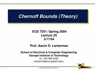
Chernoff Bounds (Gaussian Examples). ECE 7251: Spring 2004 Lecture 26 3/19/04. Prof. Aaron D. Lanterman School of Electrical & Computer Engineering Georgia Institute of Technology AL: 404-385-2548 <lanterma@ece.gatech.edu>. Main object of interest:. Both representations will be useful.

E N D
Chernoff Bounds(Gaussian Examples) ECE 7251: Spring 2004 Lecture 26 3/19/04 Prof. Aaron D. Lanterman School of Electrical & Computer Engineering Georgia Institute of Technology AL: 404-385-2548 <lanterma@ece.gatech.edu>
Main object of interest: • Both representations will be useful • Discussion based on Van Trees, pp. 126-129 Material from Last Lecture • Consider the loglikelihood ratio test
Ex. 1: What Does Mu Look Like? (Graph from p. 126 of Van Trees Vol. I)
Ex. 1: Where are the Bounds Meaningful? • Recall we need
Ex. 1: The Refined Bound for PFA • Recall the refined asymptotic bound: • In this case, since L is a sum of Gaussian random variables, the expression is exact:
Again, since L is Gaussian, the expression is exact: Ex. 1: The Refined Bound for PM Typical thing to try:Using MATLAB, plot basic Chernoff bound and true probs. of false alarm on the same graph vs. d for various choices of
Ex. 1: Minimum Prob. of Error • For minimum prob. of error test, • Recall approximate expression for Pe from last slide of last lecture
Ex. 1: Min. Prob. of Error Con’t • Recall the exact expression is: • Van Trees’ rule of thumb: “approximation is very good for d>6”
The Bhattacharyya Distance • If the criterion is the minimum prob. of error and (s) is symmetric about s=1/2, then • -(s)is called the Battacharyya distance
A common special case: EFTR: Ex. 2: Gaussian, Equal Means EFTR:
Ex. 2: What Does Mu Look Like? (Graph from p. 128 of Van Trees Vol. I)
Ex. 2: Gaussian, Equal Means EFTR: EFTR:Find an expression for the s which gives the tightest bound in terms of
Ex. 2: Gaussian, Equal Means Typical thing to do:Using MATLAB, plot four different ROC curves on the same graph: • The true curve, computed using expressions from previous lectures and built in MATLAB commands like chi2cdf, etc. • The curve given by the basic Chernoff upper bound (this gives an upper bound ROC curve) • The curve given by the asymptotic Chernoff expression using the Q functions • The curve given by the asymptotic Chernoff expression using the approximation to Q Try it for different values of n and
Ex. 2: ROC Curve Comparison (Graph from p. 129 of Van Trees Vol. I)